Fit a population model to a study, look at what the fit carries, and generate a synthetic dataset by simulating from it. Generation uses fitted population parameters and study summaries: structural curves, between-subject variability, residual error, endpoint frequencies, a planned dose schedule per arm, and dose changes and one attendance rate per endpoint, pooled over the arms. It does not read the original patient rows.
It makes no formal privacy claim, and it is not for
estimation — the fitted parameters exist to make simulated
profiles look like the source study, and the object prints that warning
with itself. The full specification is in
vignette("pmxmodel-algorithm").
The dataset is xgxr::mad: 60 patients in six treatment
arms, with a pharmacokinetic (PK) concentration endpoint and continuous,
count, ordinal and binary pharmacodynamic (PD) endpoints.
Configuration
To run this on your own study, edit the two chunks below that:
- Read in the dataset.
- Define the column roles.
The rest of the code can be kept as is.
library(dplyr)
raw <- as.data.frame(get(utils::data(list = "mad", package = "xgxr")))
SEED <- 808
The column meanings. Columns not specified here are dropped from the synthetic dataset.
roles <- pmx_roles(
  id           = "ID",
  time         = "TIME",
  dv           = "LIDV",
  mdv          = "MDV",
  amt          = "AMT",
  evid         = "EVID",
  cmt          = "CMT",
  dvid         = "NAME",        # which endpoint each observation row is
  nominal_time = "NOMTIME",     # the grid the visit model is built on
  strata       = c("TRTACT", "DOSE"), # treatment arms, fitted one at a time
  covariates   = c("WEIGHTB", "SEX") # drawn independently of the profiles
)
Fitting
synpmx_model_estimate() is the only stage that reads
patient data, and the only one that needs nlmixr2. It works
out which endpoint is the drug, what design produced it, and tries two
compartments with checked fallback to one.
fit <- synpmx_model_estimate(raw, roles, seed = 1)The chunk above is shown rather than run. Fitting compiles a model,
so this document reads a stored synpmx_model_estimate() fit
and R CMD check never needs a compiler.
The fitted clearance is 6 L/h and the volume 50 L. They put the simulated profiles where the source’s are, and are not estimates to report.
What the fit carries
model_report() prints everything the generator will
simulate from, and the diagnostics beside it.
vignette("pmxmodel-fingerprint") goes through each part,
and vignette("pmxmodel-algorithm") says how each is
estimated.
model_report(fit)
#> Summarized from the source, not estimated
#>   cohort             60 patients in 6 arm(s)
#>                      Placebo / 0 (10)
#>                      100 mg / 100 (10)
#>                      200 mg / 200 (10)
#>                      400 mg / 400 (10)
#>                      800 mg / 800 (10)
#>                      1600 mg / 1600 (10)
#>   dose changes       none
#>   visit grid         5 endpoint(s) at 28 nominal time(s), 66 slot(s) in all
#>   visit attendance   share of scheduled slots attended, one rate per
#>                      endpoint: PK Concentration 100%, PD - Continuous 100%,
#>                      PD - Count 100%, PD - Binary 100%, PD - Ordinal 100%
#>   covariates         WEIGHTB lognormal, SEX categorical, drawn once for the
#>                      whole study, independently of the profiles
#>   discrete endpoints PD - Binary, PD - Ordinal: drawn from the frequencies
#>                      of their recorded levels, not simulated
#>   columns emitted    ID, TIME, NOMTIME, LIDV, AMT, EVID, CMT, NAME, MDV,
#>                      WEIGHTB, SEX, TRTACT, DOSE
#>
#> Values at the lower limit of what was observed
#>     PK Concentration   0.02, no assay limit: half the lowest value several patients reached, rounded down
#>     PD - Continuous    0.1, no assay limit: half the lowest value several patients reached, rounded down
#>
#> Each non-PK continuous endpoint, fitted as constant, linear, or exponential
#>   PD - Continuous    exponential
#>                        plateau          30
#>                        baseline         2
#>                        rate             0.01
#>                        between-subject  1 (SD on the log baseline)
#>                        residual         additive 8
#>                        chosen on AIC from constant, linear, exponential
#>   PD - Count         exponential
#>                        plateau          3
#>                        baseline         10
#>                        rate             0.01
#>                        between-subject  0.2 (SD on the log baseline)
#>                        residual         additive 3
#>                        chosen on AIC from constant, linear, exponential
#>
#> PK endpoint for the PopPK model
#>   PK Concentration   inferred from the following data characteristics:
#>                        absent before the first dose
#>                        dose-proportional: the peak scales with the dose
#>                        recorded in the compartment the doses go into
#>                        rises to one peak and comes back down within one
#>                          dose interval
#>   route              oral: the median profile rises to a peak at 2 before
#>                      declining, and 100% of subjects do too
#>   sampling           median 13 distinct times after a dose, 9 after the
#>                      peak: richer within-subject sampling
#>
#> The PopPK model
#>
#> Estimated by nlmixr2
#>   structural model   2cmt_oral
#>   selected by        two-compartment model passed acceptance checks
#>   fitted on          all 49 patients with a concentration
#>   fixed effects      cl 6, v 50, q 5, v2 100, ka 1
#>   between-subject    cl 0.447, v 0.447, ka 0.316, q 0.548, v2 0.447 (as SD on the log scale)
#>   residual error     proportional 0.4
#>   time to fit        2 min 48 s
#>   whole call         2 min 49 s, against 2 min 48 s in the fitter
#>
#> Privacy
#>   one patient's pull pass: largest: PD - Continuous between-subject SD,
#>                      10.3 points; `model_privacy_checks()` has every check
#>   left out           1 patient(s), from the PK, PD and covariate estimates,
#>                      for moving PD - Continuous typical baseline by 16 %;
#>                      PD - Continuous between-subject SD by 23.7 points; the
#>                      dosing and visit models still read them
show(model_candidates(fit), "Models attempted and acceptance results")Generating
synpmx_model_generate() reads no patient data. Its
arguments are the fit and a subject count, so everything about the
source that reaches the output has already passed through the fit.
synthetic <- synpmx_model_generate(fit, seed = SEED)The generated table follows the declared schema: retained columns and classes, the same compartment numbers, and new identifiers.
show(head(synthetic, 10), "The first ten rows")Plot synthetic data and original data
Compare each endpoint on the recorded time scale, with source and synthetic subjects shown separately within each treatment arm.
library(ggplot2)
library(xgxr)
xgx_theme_set()
comparison_colours <- c(source = "#1B6CA8", synthetic = "#D95F02")

both <- rbind(
  cbind(raw[, names(synthetic)], DATA = "source"),
  cbind(synthetic, DATA = "synthetic")
)
obs <- both[both$EVID == 0 & !is.na(both$LIDV), ]
obs$TRTACT <- factor(obs$TRTACT,
                     levels = c("Placebo", "100 mg", "200 mg", "400 mg",
                                "800 mg", "1600 mg"))
ggplot(obs[obs$NAME == "PK Concentration" & obs$TIME <= 24, ],
       aes(TIME, LIDV, group = ID, colour = DATA)) +
  geom_line(alpha = 0.4) +
  facet_grid(DATA~TRTACT) +
  xgx_scale_y_log10() +
  xgx_scale_x_time_units("hours", breaks = seq(0, 24, by = 6)) +
  scale_colour_manual(values = comparison_colours) +
  labs(x = "Time (hours)", y = "PK concentration", colour = NULL) +
  theme(legend.position = "top") +
  ggtitle("Day 1 Conc. Profile")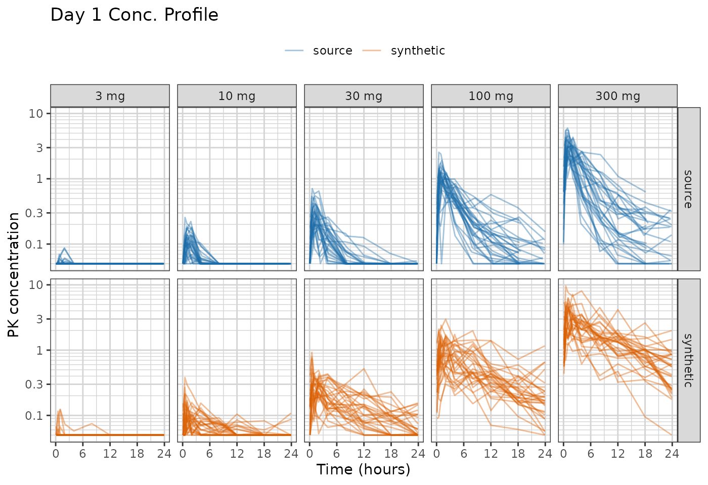
last_dose <- obs[obs$NAME == "PK Concentration" &
                   obs$TIME >= 120 & obs$TIME <= 144, ]
last_dose$TAD <- last_dose$TIME - 120

ggplot(last_dose, aes(TAD, LIDV, group = ID, colour = DATA)) +
  geom_line(alpha = 0.4) +
  facet_grid(DATA~TRTACT) +
  xgx_scale_y_log10() +
  xgx_scale_x_time_units("hours", breaks = seq(0, 24, by = 6)) +
  scale_colour_manual(values = comparison_colours) +
  labs(x = "Time after dose (hours)", y = "PK concentration", colour = NULL) +
  theme(legend.position = "top") +
  ggtitle("Last Dose (120 h) Conc. Profile")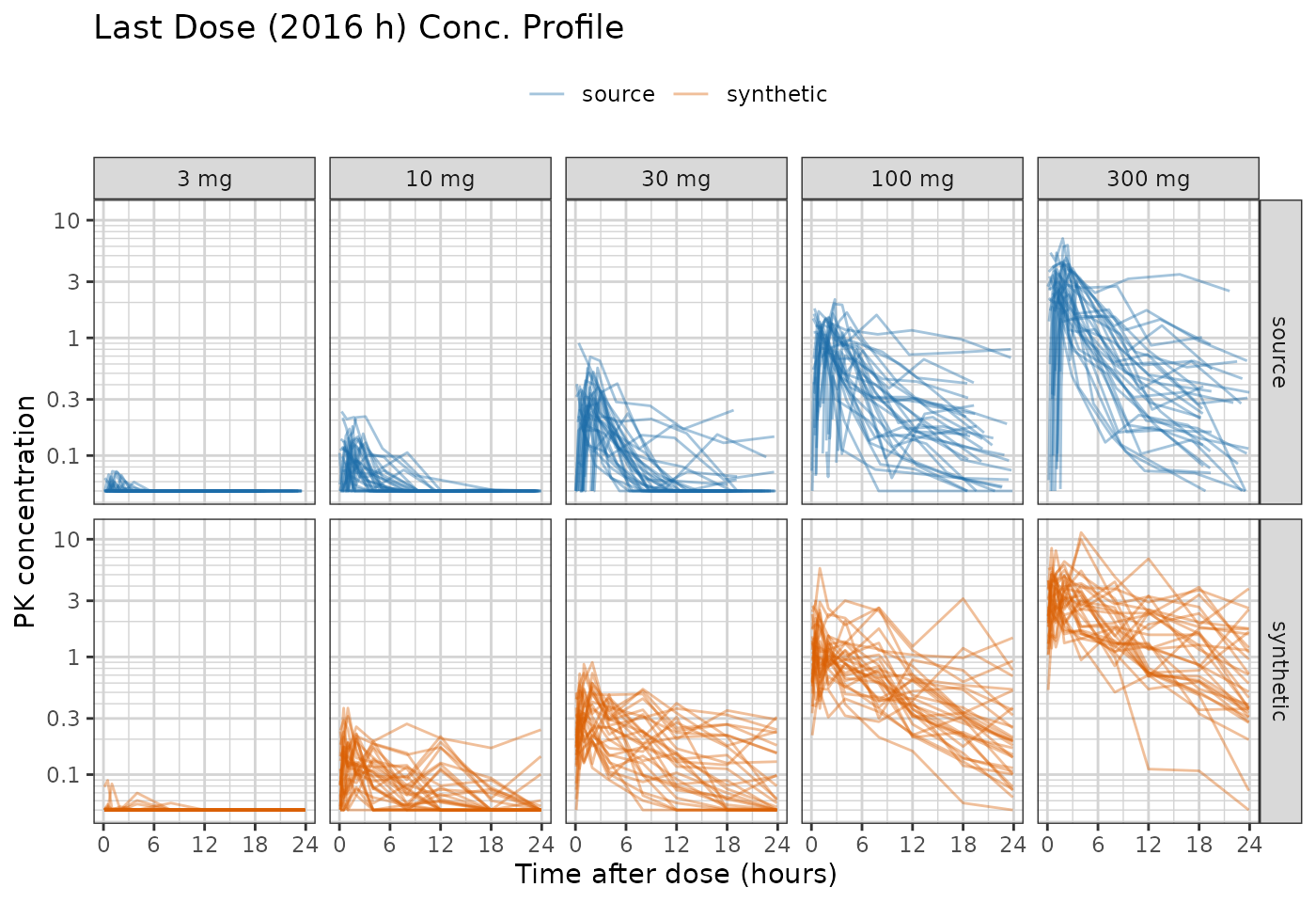
Every synthetic concentration profile uses the selected structural curve with new parameter draws and residual error. Compare the rise, decline and spread within each arm: pooled generation checks can miss discrepancies confined to one dose group or part of the sampling window.
ggplot(obs[obs$NAME == "PD - Continuous", ],
       aes(TIME, LIDV, group = ID, colour = DATA)) +
  geom_line(alpha = 0.35) +
  xgx_scale_x_time_units(units_dataset = "hours", units_plot = "days") +
  facet_grid(DATA~TRTACT) +
  scale_colour_manual(values = comparison_colours) +
  labs(x = "Time (days)", y = "PD (continuous)", colour = NULL) +
  theme(legend.position = "top") +
  ggtitle("PD Response")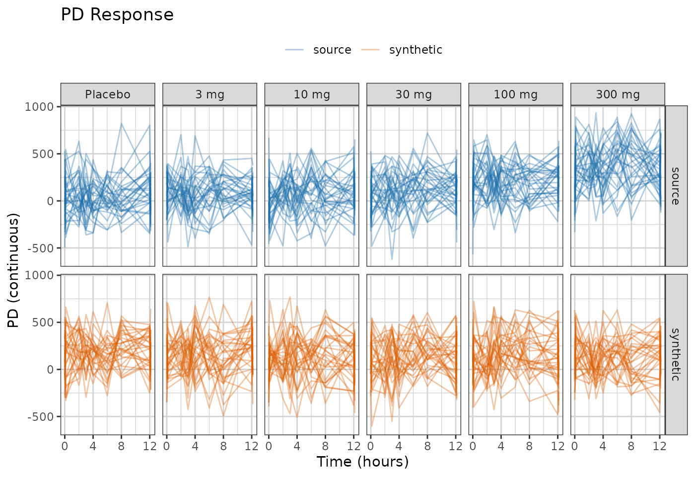
The PD time course has no exposure term, so a synthetic patient’s arm
does not reach their response. The mad section of the public-data
evaluation compares the late response by arm.
Distributions of Synthetic and Original Data
One panel per endpoint and per baseline covariate, source against
synthetic. compare_pmx_distributions_height() sizes the
figure, since it grows a row of panels at a time;
output = "tables" gives the numbers behind it.
compare_pmx_distributions(raw, synthetic, roles)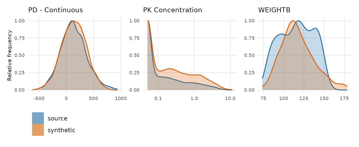
Scoring it
synpmx_scorecard() does not know what produced the
dataset it scores, so it reads this output the same way it reads an
AVATAR or PCA one.
card <- synpmx_scorecard(raw, synthetic, roles)
synpmx_scorecard_datatable(card)
Checks requiring an AVATAR run record are not applicable to this
generator. vignette("scorecard") documents what each row
asks and what its pass criterion is.
One call
synpmx_model() is the two stages together, for when you
do not need to look at the fit first. The result carries the fit’s
fingerprint as an attribute, which is what generation read; the
candidate table and the other diagnostics are only on the fit
itself.
synthetic <- synpmx_model(raw, roles, seed = SEED)
attr(synthetic, "pmx_fitted_model")
See also
-
vignette("pmxmodel-algorithm")— what each step does and why. -
vignette("pmxmodel-fingerprint")— every quantity the fit carries out of the study, in detail. - Evaluating the model generator on public data — the same generator over the public studies the other two surveys use.
-
vignette("pca-demo")— a worked study through the principal-component generator. -
vignette("avatar-demo")— a worked study through blending. -
vignette("scorecard")— the checks above, in detail. - Privacy protections in the PMX model generator — what leaves the study, and the checks on it.