Evaluating the PMX model generator on public data

This article runs synpmx_model() over the same eight public datasets that Evaluating AVATAR on public data and Evaluating PCA on public data run their generators over, so the three can be read against each other on identical studies.

This generator asks more of a study than the other two, and what separates these datasets is whether the study can identify a population model at all. Two things it will not guess, and one it will do anyway and warn about:

A declared nominal grid, as synpmx_pca() needs — the visit model is built on it. Refused, because inferring the grid is a statement about the protocol only the reader can make.
An endpoint declaration when PK inference is unsuitable. Concentration inference looks for absence before dosing and scaling with dose. A response-only study can be inferred from its positive baseline, as wbcSim is, or declared with endpoint_roles = c(pd = "DV").
A cohort large enough for a covariance matrix, which min_subjects sets at twenty. Below it the fit runs and warns: a matrix estimated from twelve subjects describes those twelve, and whether that is fit for the purpose is a judgement about the purpose rather than about the count.

wbcSim is inferred as PD-only from its baseline. nimoData needs its concentration named, and pheno_sd needs that and a nominal grid built for it, because routine care wrote none down — which is the case to read before declaring one your study does not have. theo_md needs nothing declared and warns about its twelve subjects.

Each dataset is attempted. A rejected population fit is shown as a refusal, with no synthetic data or scorecard. Successful fits follow the same generation and comparison steps.

Every fit below reads patient data once, through synpmx_model_estimate(). Generation reads only the stored fit. Comparisons and scorecards also read the source to assess the generated data.

Plotting and reporting helpers used throughout this vignette

# Observation rows only, source beside synthetic on a shared y axis, one row per
# endpoint. The same figure the PCA survey draws, so the two can be compared
# panel for panel.
# `endpoints` draws one endpoint of a study that has several. A log axis is the
# reason it exists: `facet_grid()` puts one scale on every panel, so a study
# whose concentration wants a log axis and whose PD endpoint goes negative
# cannot be one figure.
overlay_plot <- function(source, synthetic, roles, title,
                         y_label = "DV", log_y = FALSE, alpha = 0.3,
                         max_time = Inf, endpoints = NULL) {
  frame <- function(data, label) {
    observed <- as.character(data[[roles$evid]]) %in% c("0", "0.0") &
      !is.na(data[[roles$dv]])
    if (!is.null(roles$mdv)) {
      observed <- observed & as.character(data[[roles$mdv]]) %in% c("0", "0.0")
    }
    observed <- observed & as.numeric(data[[roles$time]]) <= max_time
    data.frame(
      dataset = factor(label, levels = c("Source", "Synthetic")),
      subject = as.character(data[[roles$id]][observed]),
      occasion = if (is.null(roles$occasion)) "1" else
        as.character(data[[roles$occasion]][observed]),
      time = as.numeric(data[[roles$time]][observed]),
      dv = as.numeric(data[[roles$dv]][observed]),
      endpoint = if (is.null(roles$dvid)) "DV" else
        as.character(data[[roles$dvid]][observed]),
      stringsAsFactors = FALSE
    )
  }
  plotted <- rbind(frame(source, "Source"), frame(synthetic, "Synthetic"))
  if (!is.null(endpoints)) {
    plotted <- plotted[plotted$endpoint %in% endpoints, , drop = FALSE]
  }
  figure <- ggplot2::ggplot(
    plotted,
    ggplot2::aes(time, dv,
                 group = interaction(dataset, subject, occasion),
                 colour = dataset)
  ) +
    ggplot2::geom_line(alpha = alpha) +
    ggplot2::geom_point(alpha = alpha, size = 0.7) +
    (if (length(unique(plotted$endpoint)) > 1L) {
      ggplot2::facet_grid(endpoint ~ dataset, scales = "free_y", switch = "y")
    } else {
      ggplot2::facet_wrap(~dataset)
    }) +
    ggplot2::scale_colour_manual(values = comparison_colours) +
    ggplot2::labs(x = "Time (hours)", y = y_label, title = title) +
    ggplot2::theme_minimal() +
    ggplot2::theme(legend.position = "none", strip.placement = "outside")
  if (isTRUE(log_y)) figure + ggplot2::scale_y_log10() else figure
}

overlay_height <- function(data, roles, per_endpoint = 2.2, minimum = 3.4) {
  observed <- as.character(data[[roles$evid]]) %in% c("0", "0.0")
  endpoints <- if (is.null(roles$dvid)) 1L else
    length(unique(data[[roles$dvid]][observed]))
  max(minimum, per_endpoint * endpoints)
}

# Every dataset is run the same way and its numbers collected in one place, so
# the cross-dataset tables at the end cannot drift from the sections above them.
runs <- list()
model_run <- function(label, source, roles, file, seed) {
  fit <- stored_fit(file)
  synthetic <- synpmx_model_generate(fit, seed = seed)
  runs[[label]] <<- list(label = label, source = source, roles = roles,
                         fit = fit, synthetic = synthetic,
                         card = synpmx_scorecard(source, synthetic, roles))
  invisible(runs[[label]])
}

# A scorecard row as the prose quotes it, read from the run, so a sentence
# cannot quote a number the run no longer gives.
reading <- function(label, check) {
  if (!run || is.null(runs[[label]])) return("not run here")
  card <- runs[[label]]$card
  card$result[card$check == check]
}
fails <- function(label) {
  run && !is.null(runs[[label]]) && any(runs[[label]]$card$verdict == "FAIL")
}

# Nearest-neighbour snapping onto a stated design grid, as in the PCA survey:
# which grid to snap to is a statement about the study and is written out at
# each call.
snap_to <- function(x, grid) {
  grid[max.col(-abs(outer(x, grid, "-")), ties.method = "first")]
}

case1_pkpd: six arms and a censored endpoint

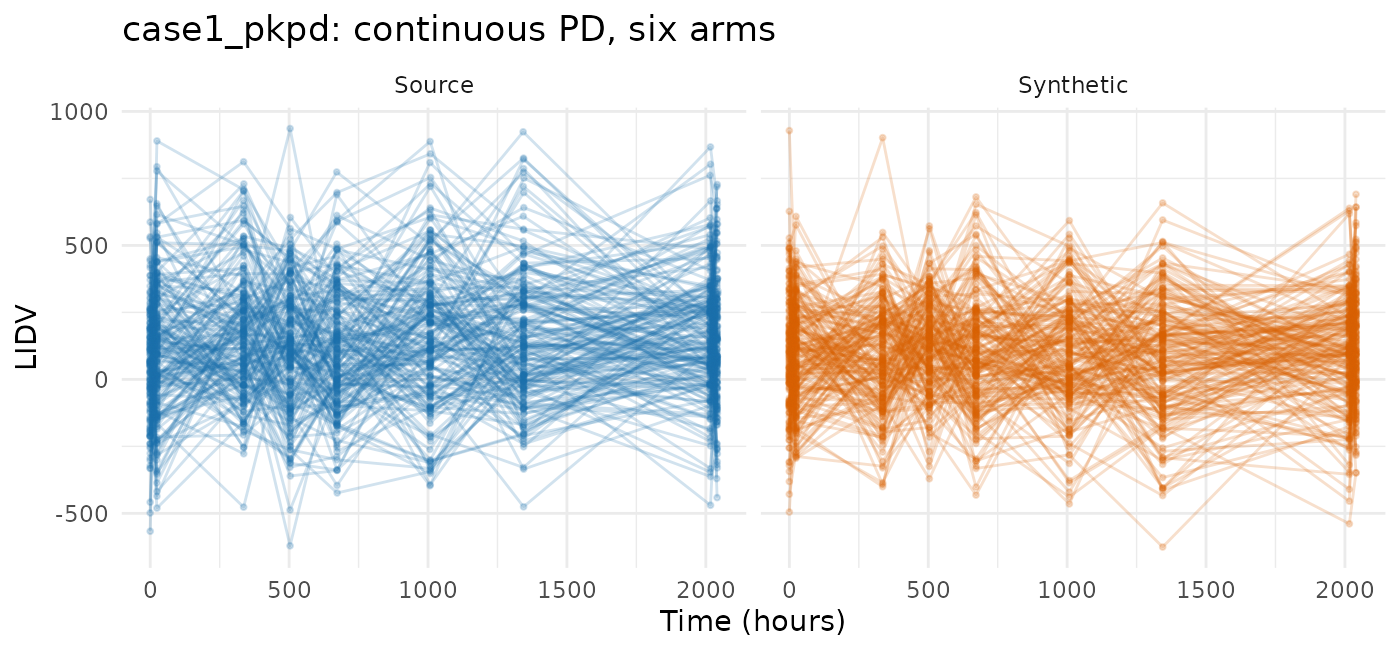
180 patients across six treatment arms, two endpoints keyed by a character NAME column, a baseline weight and a CENS column. The AVATAR and PCA demos use this study; the model demo uses mad, whose fit passed the checks.

case1_pkpd <- as.data.frame(
  get(utils::data(list = "case1_pkpd", package = "xgxr"))
)
# That study's CENS is meaningful only for PK: the PD effect is signed, so a
# left-censored PD row would report a value above the uncensored ones.
case1_pkpd$CENS <- ifelse(case1_pkpd$NAME == "PD - Continuous", 0,
                          case1_pkpd$CENS)
case1_roles <- pmx_roles(
  id = "ID", time = "TIME", dv = "LIDV", cens = "CENS", amt = "AMT",
  evid = "EVID", cmt = "CMT", dvid = "NAME", nominal_time = "NOMTIME",
  strata = c("TRTACT", "DOSE"), covariates = "WEIGHTB", keep = "STUDY"
)
case1_fit <- stored_fit("case1-pkpd-model-fit.rds")
case1 <- NULL
if (inherits(case1_fit, "pmx_example_rejection")) {
  cat(case1_fit$message, "\n")
} else {
  case1 <- model_run("case1_pkpd", case1_pkpd, case1_roles,
                     "case1-pkpd-model-fit.rds", seed = 808)
  print(case1$fit)
}
#> A fitted PMX model, from synpmx_model_estimate()
#> Everything below is an input to `synpmx_model_generate()`.
#> 
#>   candidates fitted  1 (2cmt_oral selected) 
#> 
#> Summarized from the source, not estimated
#>   cohort             180 patients in 6 arm(s)
#>                      Placebo / 0 (30)
#>                      3 mg / 3 (30)
#>                      10 mg / 10 (30)
#>                      30 mg / 30 (30)
#>                      100 mg / 100 (30)
#>                      300 mg / 300 (30)
#>   dose changes       none
#>   visit grid         2 endpoint(s) at 25 nominal time(s), 33 slot(s) in all
#>   visit attendance   share of scheduled slots attended, one rate per
#>                      endpoint: PK Concentration 100%, PD - Continuous 100%
#>   covariates         WEIGHTB lognormal, drawn once for the whole study,
#>                      independently of the profiles
#>   columns emitted    ID, TIME, NOMTIME, LIDV, AMT, EVID, CMT, NAME, CENS,
#>                      WEIGHTB, TRTACT, DOSE, STUDY
#> 
#> Values at the lower limit of what was observed
#>   Reported below the assay limit:
#>     PK Concentration   1669 of 3600 (46%) below 0.05 (the limit)
#> 
#> Each non-PK continuous endpoint, fitted as constant, linear, or exponential
#>   PD - Continuous    exponential
#>                        plateau          100
#>                        baseline         50
#>                        rate             0.05
#>                        between-subject  1 (SD on the log baseline)
#>                        residual         additive 200
#>                        chosen on AIC from constant, linear, exponential
#> 
#> PK endpoint for the PopPK model
#>   PK Concentration   inferred from the following data characteristics:
#>                        absent before the first dose
#>                        dose-proportional: the peak scales with the dose
#>                        recorded in the compartment the doses go into
#>                        rises to one peak and comes back down within one
#>                          dose interval
#>   route              oral: the median profile rises to a peak at 1 before
#>                      declining, and 99% of subjects do too
#>   sampling           median 9 distinct times after a dose, 6 after the
#>                      peak: richer within-subject sampling
#> 
#> The PopPK model
#> 
#> Estimated by nlmixr2
#>   structural model   2cmt_oral 
#>   selected by        two-compartment model passed acceptance checks
#>   fit checks         Warning: the optimizer stalled before convergence was
#>                      confirmed. Check that the synthetic data reasonably
#>                      reproduces the source data's patterns and
#>                      variability.; median checked against censoring bounds;
#>                      spread comparison omitted for censored observations
#>   fitted on          60 of 150 patients with a concentration, drawn in
#>                      proportion to the arms under `max_fit_subjects` = 60;
#>                      the dosing, visit and covariate models below read the
#>                      whole study
#>   fixed effects      cl 10, v 60, q 8, v2 200, ka 2 
#>   between-subject    cl 0.447, v 0.316, ka 0.1, q 0.1, v2 0.1 (as SD on the log scale)
#>   starting values    cl 13, v 65, q 8, v2 150, ka 2 declared through
#>                      `start_param`; the rest were read off the cohort's
#>                      median profile
#>   residual error     proportional 0.3 
#>   time to fit        19 min 18 s
#>   whole call         19 min 20 s, against 19 min 18 s in the fitter
#> 
#> Privacy
#>   one patient's pull pass: largest: PD - Continuous between-subject SD,
#>                      6.44 points; `model_privacy_checks()` has every check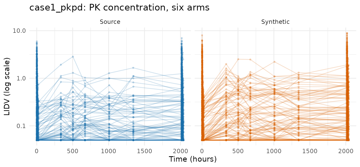

compare_pmx_distributions(case1$source, case1$synthetic, case1_roles)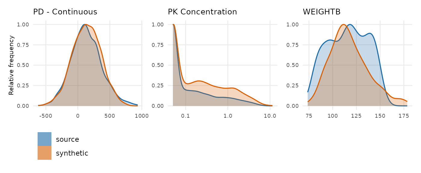

synpmx_scorecard_datatable(case1$card, report = "minimal")

The stored fit uses start_param = c(cl = 13, v = 65, q = 8, v2 = 150, ka = 2), rounded starts from an exploratory fit of this public study. The two-compartment fit reports false convergence. That warning remains in the candidate table; the fit passes the parameter and generation checks and is used for this synthetic cohort. No one-compartment fallback is needed. vignette("pmxmodel-demo") uses mad for the end-to-end example.

Five rows read not applicable on every card in this article. The cards below count them in their tally and do not list them, so they are worth reading once here. B1a, B1b and C2 need a run record that synpmx_avatar() writes and this generator does not. B4a asks whether a generated set of observation times copies a real one, which is a disclosure question only where the set was taken from somebody: this generator decides each visit independently, at its endpoint’s attendance rate, so a match is a coincidence with a computable chance. B2 asks whether a synthetic patient stands out from its stratum, which is a disclosure question for a generator that hands a real patient’s trajectory to an avatar and a reading about the tail of a distribution here. B4b is the row that carries the claim here, and it is 0 on every dataset below: no value any patient measured is reproduced.

mad: five endpoints, only one of them a concentration

60 subjects in a multiple-ascending-dose study with a declared NOMTIME and five endpoints — PK concentration, continuous PD, and ordinal, count and binary PD. The generator fits a structural model to the concentration and a shape to each continuous PD endpoint; the discrete ones are a question this generator does not answer.

mad <- as.data.frame(get(utils::data(list = "mad", package = "xgxr")))
mad_roles <- pmx_roles(
  id = "ID", time = "TIME", dv = "LIDV", amt = "AMT", evid = "EVID",
  cmt = "CMT", dvid = "NAME", mdv = "MDV", nominal_time = "NOMTIME",
  strata = c("TRTACT", "DOSE"), covariates = c("WEIGHTB", "SEX")
)
mad_run <- model_run("mad", mad, mad_roles, "mad-model-fit.rds", seed = 909)
mad_run$fit
#> A fitted PMX model, from synpmx_model_estimate()
#> Everything below is an input to `synpmx_model_generate()`.
#> 
#>   candidates fitted  1 (2cmt_oral selected) 
#> 
#> Summarized from the source, not estimated
#>   cohort             60 patients in 6 arm(s)
#>                      Placebo / 0 (10)
#>                      100 mg / 100 (10)
#>                      200 mg / 200 (10)
#>                      400 mg / 400 (10)
#>                      800 mg / 800 (10)
#>                      1600 mg / 1600 (10)
#>   dose changes       none
#>   visit grid         5 endpoint(s) at 28 nominal time(s), 66 slot(s) in all
#>   visit attendance   share of scheduled slots attended, one rate per
#>                      endpoint: PK Concentration 100%, PD - Continuous 100%,
#>                      PD - Count 100%, PD - Binary 100%, PD - Ordinal 100%
#>   covariates         WEIGHTB lognormal, SEX categorical, drawn once for the
#>                      whole study, independently of the profiles
#>   discrete endpoints PD - Binary, PD - Ordinal: drawn from the frequencies
#>                      of their recorded levels, not simulated
#>   columns emitted    ID, TIME, NOMTIME, LIDV, AMT, EVID, CMT, NAME, MDV,
#>                      WEIGHTB, SEX, TRTACT, DOSE
#> 
#> Values at the lower limit of what was observed
#>     PK Concentration   0.02, no assay limit: half the lowest value several patients reached, rounded down
#>     PD - Continuous    0.1, no assay limit: half the lowest value several patients reached, rounded down
#> 
#> Each non-PK continuous endpoint, fitted as constant, linear, or exponential
#>   PD - Continuous    exponential
#>                        plateau          30
#>                        baseline         2
#>                        rate             0.01
#>                        between-subject  1 (SD on the log baseline)
#>                        residual         additive 8
#>                        chosen on AIC from constant, linear, exponential
#>   PD - Count         exponential
#>                        plateau          3
#>                        baseline         10
#>                        rate             0.01
#>                        between-subject  0.2 (SD on the log baseline)
#>                        residual         additive 3
#>                        chosen on AIC from constant, linear, exponential
#> 
#> PK endpoint for the PopPK model
#>   PK Concentration   inferred from the following data characteristics:
#>                        absent before the first dose
#>                        dose-proportional: the peak scales with the dose
#>                        recorded in the compartment the doses go into
#>                        rises to one peak and comes back down within one
#>                          dose interval
#>   route              oral: the median profile rises to a peak at 2 before
#>                      declining, and 100% of subjects do too
#>   sampling           median 13 distinct times after a dose, 9 after the
#>                      peak: richer within-subject sampling
#> 
#> The PopPK model
#> 
#> Estimated by nlmixr2
#>   structural model   2cmt_oral 
#>   selected by        two-compartment model passed acceptance checks
#>   fitted on          all 49 patients with a concentration
#>   fixed effects      cl 6, v 50, q 5, v2 100, ka 1 
#>   between-subject    cl 0.447, v 0.447, ka 0.316, q 0.548, v2 0.447 (as SD on the log scale)
#>   residual error     proportional 0.4 
#>   time to fit        2 min 48 s
#>   whole call         2 min 49 s, against 2 min 48 s in the fitter
#> 
#> Privacy
#>   one patient's pull pass: largest: PD - Continuous between-subject SD,
#>                      10.3 points; `model_privacy_checks()` has every check
#>   left out           1 patient(s), from the PK, PD and covariate estimates,
#>                      for moving PD - Continuous typical baseline by 16 %;
#>                      PD - Continuous between-subject SD by 23.7 points; the
#>                      dosing and visit models still read them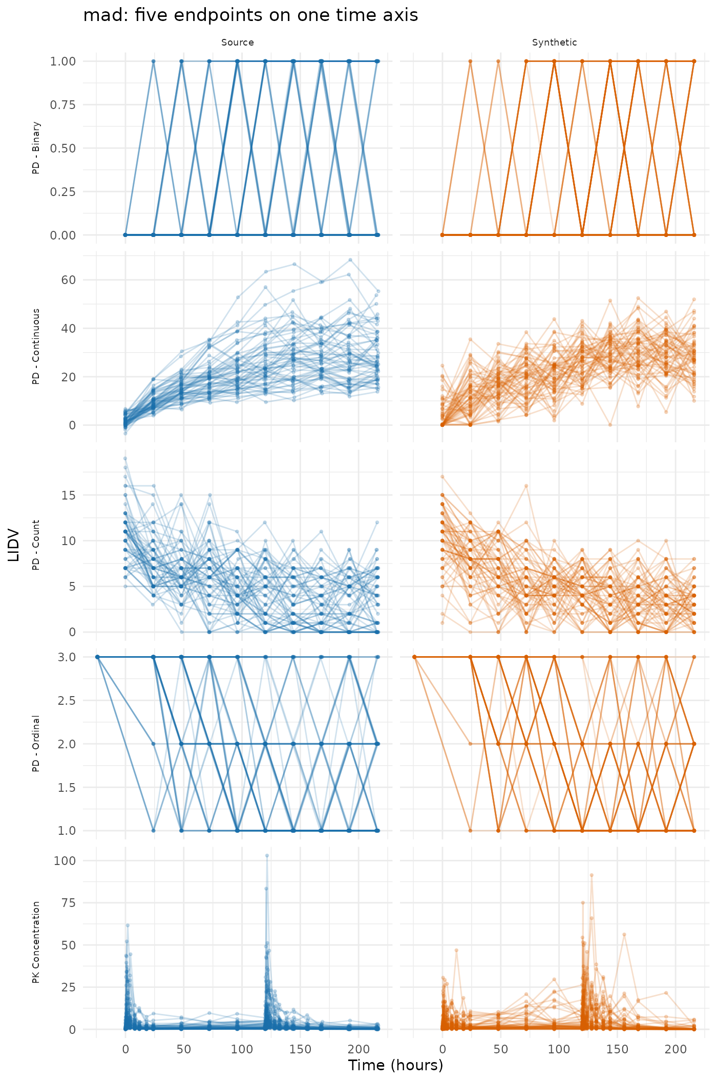

synpmx_scorecard_datatable(mad_run$card, report = "minimal")

Nothing fails, and A3 reads 5 of 5: every endpoint survives, including the three discrete ones, which are drawn from one set of level frequencies for the whole study rather than modelled. Pooled, a discrete endpoint’s response differs neither by dose group, as the continuous PD time course already does not, nor over the visits. D1 reads sd x0.74 on PK Concentration (furthest of 6), the variable whose synthetic spread sits furthest from the source’s.

The continuous PD time course has no exposure term, so the dose ordering of the response is lost. The mean response after the last dose, by arm:

late_pd <- function(data, label) {
  rows <- data$NAME == "PD - Continuous" & data$EVID == 0 &
    data$TIME > 144 & !is.na(data$LIDV)
  out <- aggregate(list(mean_pd = data$LIDV[rows]),
                   list(arm = data$TRTACT[rows]), function(x) signif(mean(x), 3))
  stats::setNames(out, c("arm", paste0("mean_pd_", label)))
}
knitr::kable(merge(late_pd(mad_run$source, "source"),
                   late_pd(mad_run$synthetic, "synthetic"), by = "arm"))

arm	mean_pd_source	mean_pd_synthetic
100 mg	25.6	29.8
1600 mg	37.3	22.7
200 mg	26.3	26.3
400 mg	31.5	27.9
800 mg	34.0	25.1
Placebo	16.3	24.1

pd_by_arm = TRUE fits the shape within each arm and would keep the ordering between arms, without saying anything about exposure within one.

This is also the study that found a defect: a visit where every patient recorded the same level of an ordinal endpoint left the draw with a single level, and the draw read that level as a count of levels rather than as the level itself. Fixed, and pinned by a regression test.

warfarin: a single dose, and no dose levels to compare

32 subjects, a single oral dose, a PK endpoint (cp) and a PD one (pca) on different time courses. Its 16 recorded observation times are the protocol’s, so declaring nominal_time from time states something true about this study rather than constructing a grid.

data("warfarin", package = "nlmixr2data")
warfarin <- as.data.frame(warfarin)
warfarin$ntime <- warfarin$time
warfarin_roles <- pmx_roles(
  id = "id", time = "time", nominal_time = "ntime", dv = "dv", amt = "amt",
  evid = "evid", dvid = "dvid", covariates = c("wt", "age", "sex")
)
warfarin_run <- model_run("warfarin", warfarin, warfarin_roles,
                          "warfarin-model-fit.rds", seed = 404)
model_report(warfarin_run$fit)
#> Summarized from the source, not estimated
#>   cohort             32 patients in 1 arm(s)
#>                      all (32)
#>   dose changes       none
#>   visit grid         2 endpoint(s) at 16 nominal time(s), 22 slot(s) in all
#>   visit attendance   share of scheduled slots attended, one rate per
#>                      endpoint: cp 55%, pca 91%
#>   covariates         wt lognormal, age lognormal, sex categorical, drawn
#>                      once for the whole study, independently of the
#>                      profiles
#>   columns emitted    id, time, ntime, dv, amt, evid, dvid, wt, age, sex
#> 
#> Values at the lower limit of what was observed
#>     cp                 0.2, no assay limit: half the lowest value several patients reached, rounded down
#>     pca                5, no assay limit: half the lowest value several patients reached, rounded down
#> 
#> Each non-PK continuous endpoint, fitted as constant, linear, or exponential
#>   pca                exponential
#>                        plateau          30
#>                        baseline         100
#>                        rate             0.1
#>                        between-subject  0.1 (SD on the log baseline)
#>                        residual         additive 10
#>                        chosen on AIC from constant, linear, exponential
#> 
#> PK endpoint for the PopPK model
#>   cp                 inferred from the following data characteristics:
#>                        absent before the first dose
#>                        rises to one peak and comes back down within one
#>                          dose interval
#>   route              oral: the median profile rises to a peak at 9 before
#>                      declining, and 31% of subjects do too
#>   sampling           median 6 distinct times after a dose, 6 after the
#>                      peak: sparse within-subject sampling
#> 
#> The PopPK model
#> 
#> Estimated by nlmixr2
#>   structural model   2cmt_oral 
#>   selected by        two-compartment model passed acceptance checks
#>   fitted on          all 32 patients with a concentration
#>   fixed effects      cl 0.1, v 7, q 0.1, v2 2, ka 0.4 
#>   between-subject    cl 0.265, v 0.2, ka 0.548, q 0.0775, v2 0.632 (as SD on the log scale)
#>   residual error     proportional 0.2 
#>   time to fit        50.9 s
#>   whole call         51.1 s, against 50.9 s in the fitter
#> 
#> Privacy
#>   one patient's pull pass: largest: cp: ka between-subject SD, 9.84 points;
#>                      `model_privacy_checks()` has every check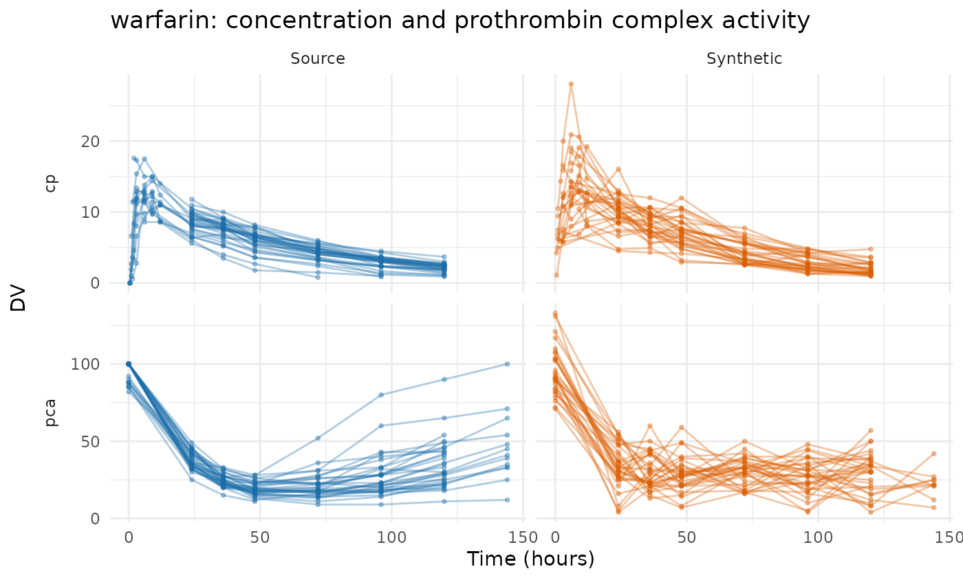

compare_pmx_distributions(warfarin_run$source, warfarin_run$synthetic,
                          warfarin_roles)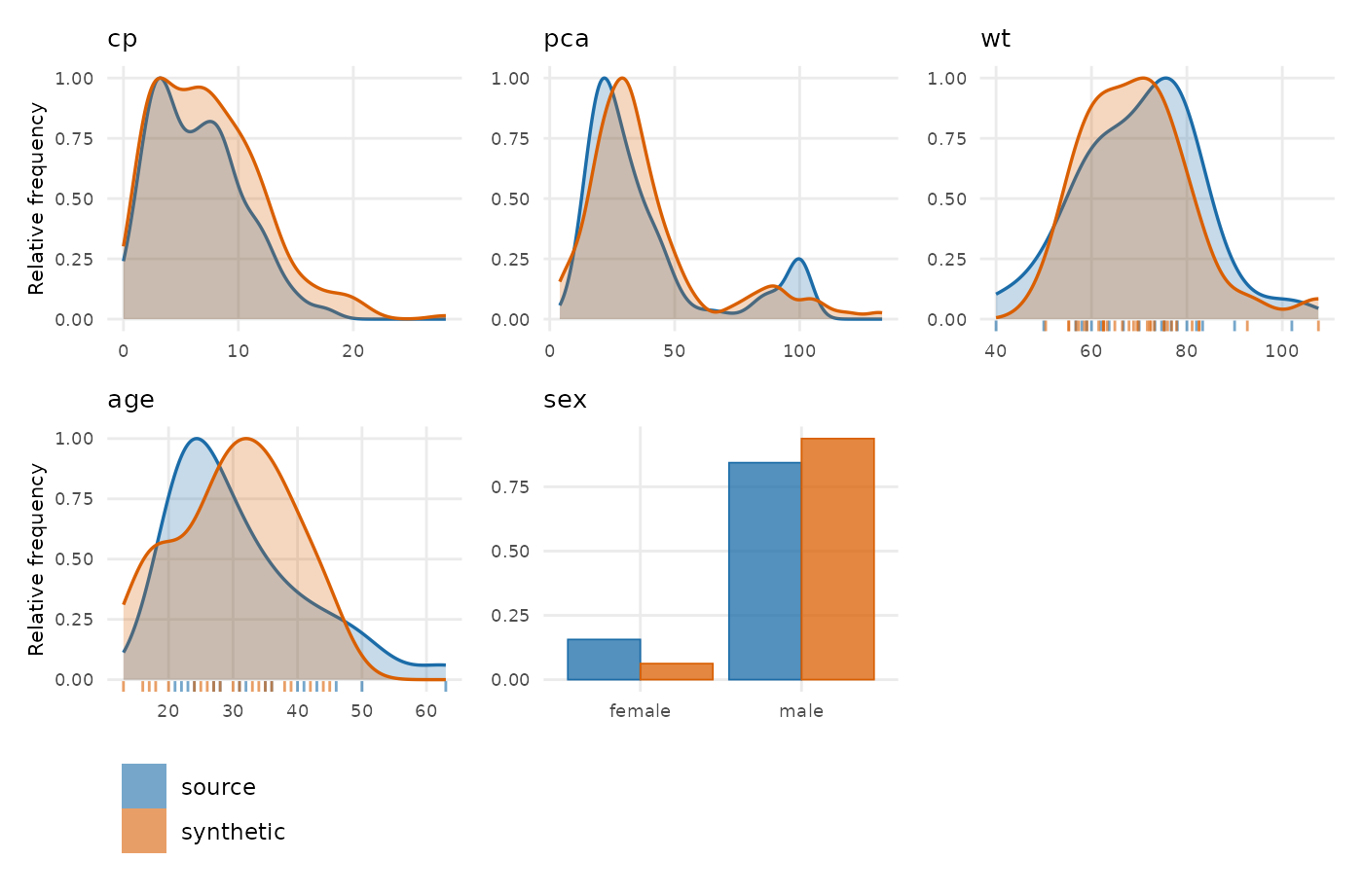

synpmx_scorecard_datatable(warfarin_run$card, report = "minimal")

Read the design line in the report above rather than the parameters. It says the median profile peaks at 9 h and that 31% of subjects do too — 22 of the 32 are first sampled at 24 h, well past the peak, so most individual profiles only decline. The route was decided from the pooled median rather than by a per-subject vote for exactly that reason, and the low percentage is the fit telling you how much it had to go on. proportional reads NA for the same kind of reason: every patient gets the same dose, so there are no dose levels to compare and the residual error falls back to additive.

Nothing fails; D1 reads sd x0.81 on wt (furthest of 4). The concentration panel of the figure is the generator at its best on this survey — the shape, the spread and the decline all land.

The pca panel below it is the generator at its documented limit. The source’s prothrombin activity falls to a nadir and comes back: median 100, 32, 18, 22, 35 over the first 12 hours, then to 36, 60, 100 and beyond 100 hours. The synthetic reads 91, 31, 28, 29, 30 — it falls and then flattens. The PD shapes are constant, linear and exponential fitted to the pooled observations, and none of the three can come back up.

wbcSim: an infusion and a delayed response

45 subjects with infusion start/stop pairs and a delayed white-blood-cell decline, nadir and recovery. The concentration this generator looks for is not here: what is recorded is the response.

data("wbcSim", package = "nlmixr2data")
wbcSim <- as.data.frame(wbcSim)
wbcSim$NTIME <- wbcSim$TIME
wbc_roles <- pmx_roles(
  id = "ID", time = "TIME", nominal_time = "NTIME", dv = "DV", amt = "AMT",
  evid = "EVID", cmt = "CMT", rate = "RATE"
)
# The positive baseline identifies this as a PD-only study.
wbc_run <- model_run("wbcSim", wbcSim, wbc_roles, "wbcsim-model-fit.rds",
                     seed = 505)
print(model_report(wbc_run$fit))
#> Summarized from the source, not estimated
#>   cohort             45 patients in 1 arm(s)
#>                      all (45)
#>   dose routes        one route, undeclared; infused over 1 h
#>   dose changes       none
#>   visit grid         1 endpoint(s) at 11 nominal time(s), 11 slot(s) in all
#>   visit attendance   share of scheduled slots attended, one rate per
#>                      endpoint: DV 28%
#>   columns emitted    ID, TIME, NTIME, DV, AMT, EVID, CMT, RATE
#> 
#> Values at the lower limit of what was observed
#>     DV                 0.2, no assay limit: half the lowest value several patients reached, rounded down
#> 
#> Each non-PK continuous endpoint, fitted as constant, linear, or exponential
#>   DV                 constant
#>                        baseline         7
#>                        between-subject  0.4 (SD on the log baseline)
#>                        residual         additive 3
#>                        chosen on AIC from constant, linear
#> 
#> PD-only study: no PK model fitted. Responses use study-time shapes or visit frequencies.
#>   whole call         0.0 s, against 0.0 s in the fitter
#> 
#> Privacy
#>   one patient's pull pass: largest: DV between-subject SD, 2.39 points;
#>                      `model_privacy_checks()` has every check
#>   left out           1 patient(s), from the PK, PD and covariate estimates,
#>                      for moving DV slope by 241 %; the dosing and visit
#>                      models still read them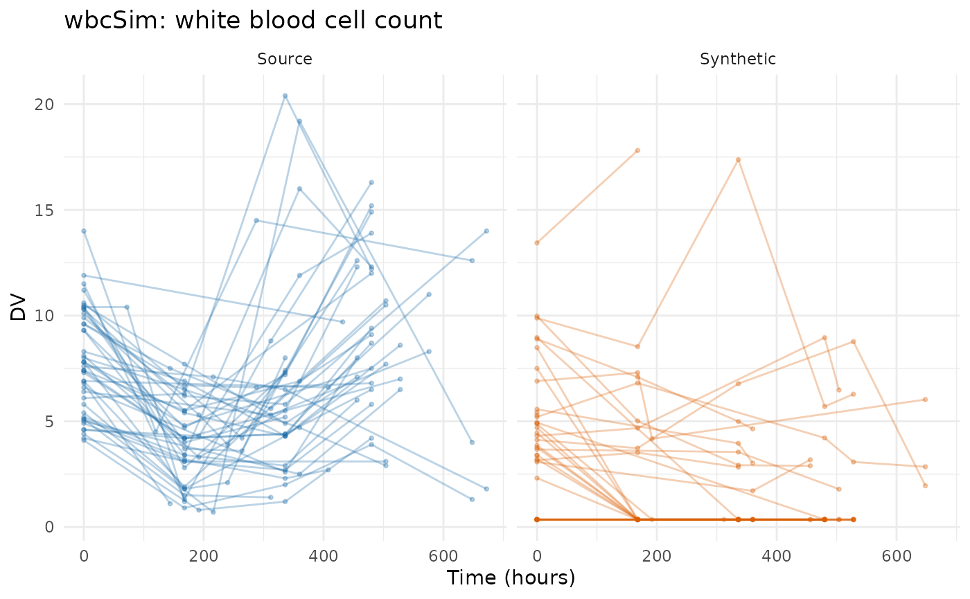

compare_pmx_distributions(wbc_run$source, wbc_run$synthetic, wbc_roles)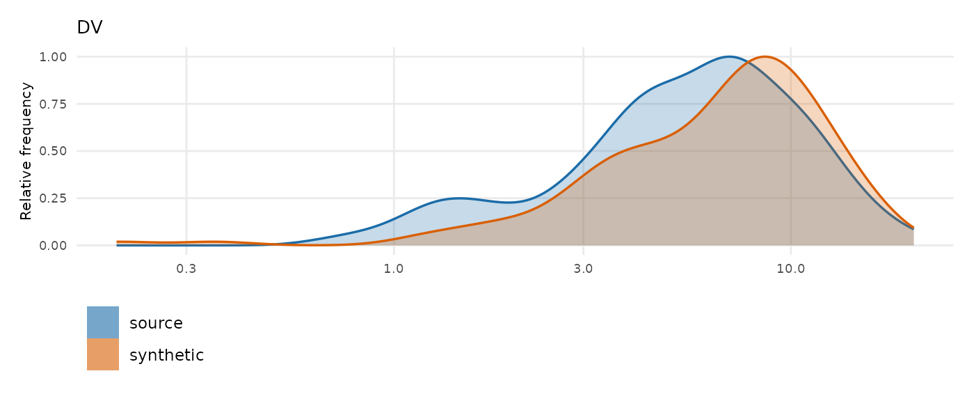

synpmx_scorecard_datatable(wbc_run$card, report = "minimal")

The positive first-dose baseline identifies this as a PD-only study. No compartment model is attempted. The report shows the response’s time-course fit and its residual variation, alongside the infusion and visit summaries.

The available PD shapes cannot reproduce a decline followed by recovery. Accepting a PD-only study makes the endpoint classification correct; it does not make this simple time-course catalogue a cell-turnover model. Read the source-versus-synthetic plot for that missing shape.

mavoglurant: an occasion-reset clock

120 subjects in one- and two-period profiles, with TIME resetting inside OCC so it is already dose-relative. The grid is the one the PCA survey writes down, reused unchanged.

data("mavoglurant", package = "nlmixr2data")
mavoglurant <- as.data.frame(mavoglurant)
mavo_design <- c(0, 0.25, 0.5, 0.75, 1, 1.5, 2, 3, 4, 6, 8, 10, 12, 24, 36, 48)
mavoglurant$NTIME <- ifelse(mavoglurant$EVID == 0,
                            snap_to(mavoglurant$TIME, mavo_design),
                            mavoglurant$TIME)
mavo_roles <- pmx_roles(
  id = "ID", time = "TIME", nominal_time = "NTIME", dv = "DV", amt = "AMT",
  evid = "EVID", cmt = "CMT", rate = "RATE", mdv = "MDV", occasion = "OCC",
  keep = "DOSE", covariates = c("AGE", "SEX", "WT", "HT")
)
mavo_run <- model_run("mavoglurant", mavoglurant, mavo_roles,
                      "mavoglurant-model-fit.rds", seed = 707)
#> Warning: 9% of generated observations (116 of 1343) fell below the emission floor
#> and were raised to it.
#>   A floor catching this much is a fitted model that does not describe the
#>   low end of the data, not an assay limit.
#>   Fix: Read `model_report()` before using this dataset.
mavo_run$fit
#> A fitted PMX model, from synpmx_model_estimate()
#> Everything below is an input to `synpmx_model_generate()`.
#> 
#>   candidates fitted  1 (2cmt_infusion selected) 
#> 
#> Summarized from the source, not estimated
#>   cohort             120 patients in 1 arm(s)
#>                      all (120)
#>   dose routes        one route, undeclared; infused over 0.1667 h
#>   dose changes       none
#>   visit grid         1 endpoint(s) at 14 nominal time(s), 14 slot(s) in all
#>   visit attendance   share of scheduled slots attended, one rate per
#>                      endpoint: DV 80%
#>   covariates         AGE lognormal, SEX lognormal, WT lognormal, HT
#>                      lognormal, drawn once for the whole study,
#>                      independently of the profiles
#>   columns emitted    ID, TIME, NTIME, OCC, DV, AMT, EVID, CMT, MDV, RATE,
#>                      AGE, SEX, WT, HT, DOSE
#> 
#> Values at the lower limit of what was observed
#>     DV                 1, no assay limit: half the lowest value several patients reached, rounded down
#> 
#> PK endpoint for the PopPK model
#>   DV                 inferred from the following data characteristics:
#>                        absent before the first dose
#>                        dose-proportional: the peak scales with the dose
#>                        recorded in the compartment the doses go into
#>                        rises to one peak and comes back down within one
#>                          dose interval
#>   route              infusion: a nonzero `rate` on the dose records
#>   sampling           median 11 distinct times after a dose, 10 after the
#>                      peak: richer within-subject sampling
#> 
#> The PopPK model
#> 
#> Estimated by nlmixr2
#>   structural model   2cmt_infusion 
#>   selected by        two-compartment model passed acceptance checks
#>   fitted on          60 of 120 patients with a concentration, drawn in
#>                      proportion to the arms under `max_fit_subjects` = 60;
#>                      the dosing, visit and covariate models below read the
#>                      whole study
#>   fixed effects      cl 0.04, v 0.1, q 0.05, v2 0.2 
#>   between-subject    cl 0.316, v 0.447, q 0.316, v2 0.447 (as SD on the log scale)
#>   residual error     proportional 0.3 
#>   time to fit        37.9 s
#>   whole call         38.1 s, against 37.9 s in the fitter
#> 
#> Privacy
#>   one patient's pull pass: largest: DV: v2 between-subject SD, 2.09 points;
#>                      `model_privacy_checks()` has every check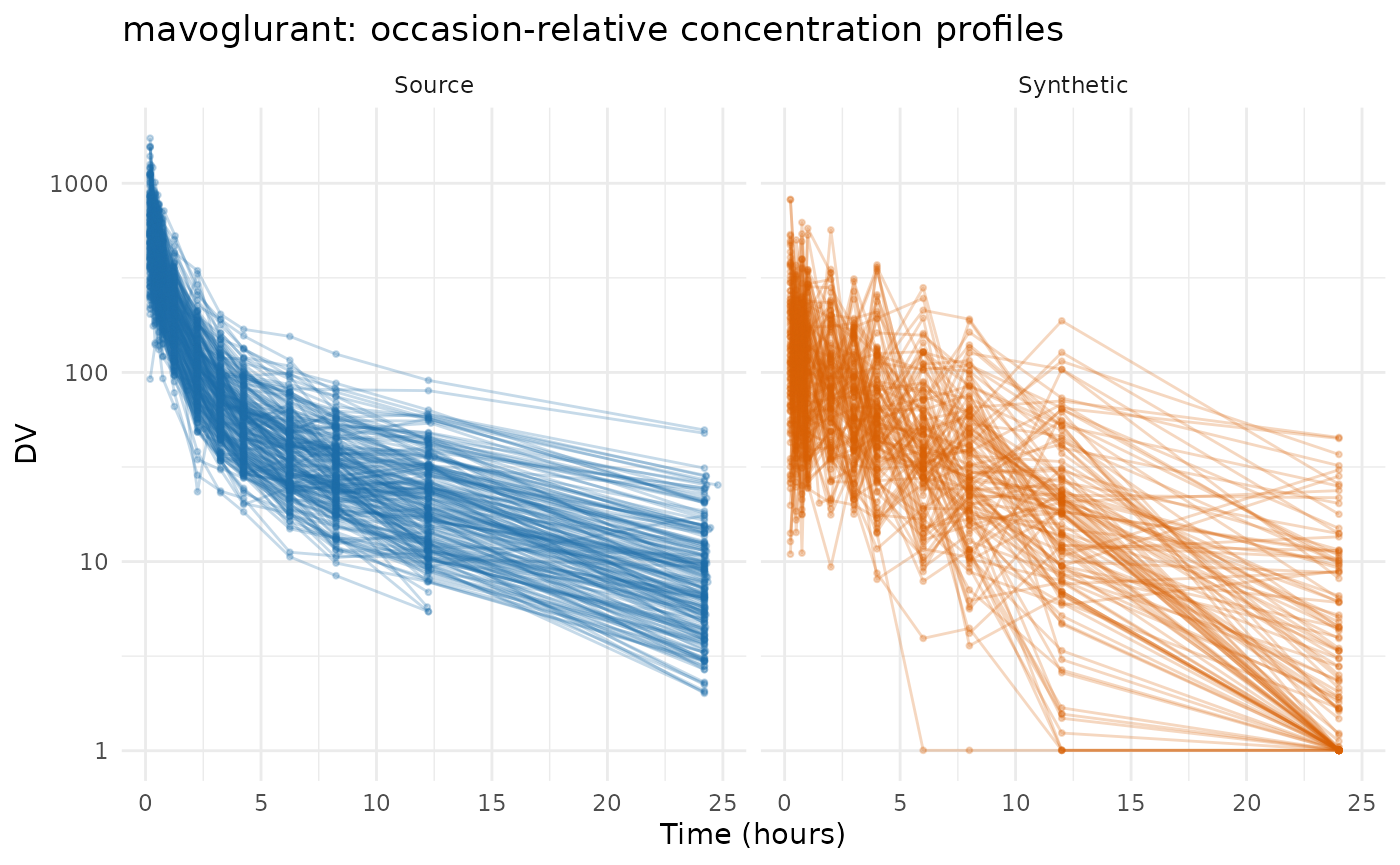

synpmx_scorecard_datatable(mavo_run$card, report = "minimal")

Three rows to read, and two findings. A5b reports occasions per patient at 1.65 -> 1 and A5a observations per patient at 20.2 -> 11.2: mavoglurant is one- and two-period, and the dosing model carries one planned schedule per arm, so the patients who had a second period do not get it back. A study whose periods matter needs them declared as arms, or a generator that keeps each patient’s own schedule.

The second finding used to be in the figure rather than the card, and this is the study that closed it. The source’s profiles are a tight declining band, the synthetic ones scattered across it, and a line of values sat on the assay floor. The cause was the candidate set. A rate role makes this an infusion study, and the closed-form set held two compartments for a bolus and for an oral dose and not for an infusion — so a drug with an obvious distribution phase was fitted a one-compartment model, which took a proportional residual of 0.72 and wrote that scatter into every generated value. 2cmt_infusion is now in the set and tried first by default. The report above gives the accepted model, its residual error, and any fallback reason.

The scorecard moves less than the fit does. D1 reads sd x0.38 on DV (furthest of 5), and A5a and A5b do not move at all, because what they measure is the visit and dosing models rather than the structural one. A better-fitting structural model is a fit-quality argument here rather than a scorecard one.

theo_md: twelve subjects, which is below the floor

12 subjects, seven doses exactly 24 h apart, dense sampling around the first and last dose. The grid is constructible and the endpoint is a concentration, so nothing stands between this study and a fit except the cohort size — and that is a warning rather than a refusal.

data("theo_md", package = "nlmixr2data")
theo_md <- as.data.frame(theo_md)
theo_doses <- seq(0, 144, by = 24)
theo_samples <- c(0, 0.25, 0.5, 1, 2, 3, 4, 5, 7, 9, 12, 24)
interval <- pmax(1L, findInterval(theo_md$TIME, theo_doses))
theo_md$NTIME <- ifelse(
  theo_md$EVID == 0,
  theo_doses[interval] +
    snap_to(theo_md$TIME - theo_doses[interval], theo_samples),
  theo_md$TIME
)
theo_roles <- pmx_roles(
  id = "ID", time = "TIME", nominal_time = "NTIME", dv = "DV", amt = "AMT",
  evid = "EVID", cmt = "CMT", covariates = "WT"
)

synpmx_model_estimate(theo_md, theo_roles, seed = 1) fits, and says what it is doing on the way past:

synpmx_model_estimate() is fitting a population model to 12 subjects, below min_subjects = 20. The fixed effects and the covariance matrix describe those 12 subjects rather than a population, and nothing downstream will tell you so: the scorecard asks whether the output copies anybody or changed the study’s shape, and a small-cohort fit does neither.

The floor is an argument rather than a constant, so min_subjects = 12L says the consequence is understood and silences it. That is what the stored fit below was built with, and what it costs is stated in the row it fills in the closing tables: a covariance matrix estimated from twelve subjects describes those twelve.

theo_run <- model_run("theo_md", theo_md, theo_roles, "theo-md-model-fit.rds",
                      seed = 303)
theo_run$fit
#> A fitted PMX model, from synpmx_model_estimate()
#> Everything below is an input to `synpmx_model_generate()`.
#> 
#>   candidates fitted  1 (2cmt_oral selected) 
#> 
#> Summarized from the source, not estimated
#>   cohort             12 patients in 1 arm(s)
#>                      all (12)
#>   dose changes       none
#>   visit grid         1 endpoint(s) at 25 nominal time(s), 25 slot(s) in all
#>   visit attendance   share of scheduled slots attended, one rate per
#>                      endpoint: DV 87%
#>   covariates         WT lognormal, drawn once for the whole study,
#>                      independently of the profiles
#>   columns emitted    ID, TIME, NTIME, DV, AMT, EVID, CMT, WT
#> 
#> Values at the lower limit of what was observed
#>     DV                 0.2, no assay limit: half the lowest value several patients reached, rounded down
#> 
#> PK endpoint for the PopPK model
#>   DV                 inferred from the following data characteristics:
#>                        absent before the first dose
#>                        recorded in the compartment the doses go into
#>                        rises to one peak and comes back down within one
#>                          dose interval
#>   route              oral: the median profile rises to a peak at 2 before
#>                      declining, and 100% of subjects do too
#>   sampling           median 11 distinct times after a dose, 6 after the
#>                      peak: richer within-subject sampling
#> 
#> The PopPK model
#> 
#> Estimated by nlmixr2
#>   structural model   2cmt_oral 
#>   selected by        two-compartment model passed acceptance checks
#>   fit checks         Warning: the optimizer stalled before convergence was
#>                      confirmed. Check that the synthetic data reasonably
#>                      reproduces the source data's patterns and variability.
#>   fitted on          all 12 patients with a concentration
#>   fixed effects      cl 3, v 30, q 2, v2 4, ka 1 
#>   between-subject    cl 0.2, v 0.141, ka 0.548, q 0.245, v2 0.283 (as SD on the log scale)
#>   residual error     proportional 0.2 
#>   time to fit        46.1 s
#>   whole call         46.1 s, against 46.1 s in the fitter
#> 
#> Privacy
#>   one patient's pull pass: largest: DV: ka typical value, 9.92 %;
#>                      `model_privacy_checks()` has every check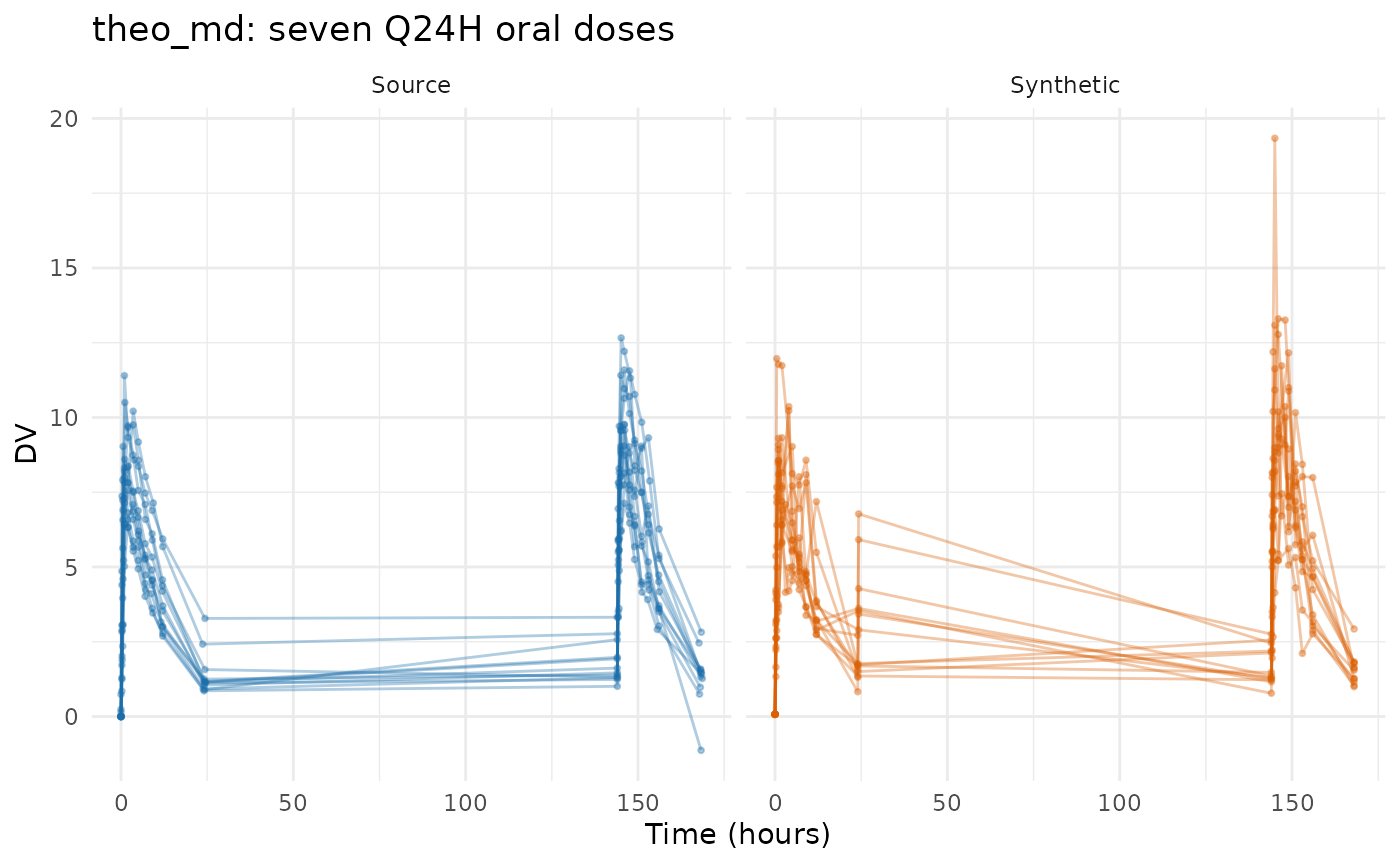

synpmx_scorecard_datatable(theo_run$card, report = "minimal")

Nothing fails, and the card looks like the others. That is the uncomfortable part: the scorecard cannot see that a covariance matrix came from twelve subjects, because the question it asks is whether this output copies anybody or changed the study’s shape, and a twelve-subject fit does neither. The floor exists because nothing downstream of it can tell.

nimoData: the endpoint has to be named

12 subjects, ten roughly weekly infusions, with dose times recorded as actuals. The grid construction is the one the AVATAR and PCA surveys work out, reused unchanged. Its twelve subjects draw the same warning theo_md did, and then it is refused for a reason worth reading.

data("nimoData", package = "nlmixr2data")
nimoData <- as.data.frame(nimoData)
nimo_interval <- 168
last_occasion <- ave(nimoData$OCC, nimoData$ID, FUN = max)
nominal_tad <- round(nimoData$TAD / 24) * 24
pre_dose <- nimoData$EVID == 0 & nominal_tad >= nimo_interval &
  nimoData$OCC < last_occasion
nominal_tad[pre_dose] <- nimo_interval - 1
nimoData$NTIME <- (nimoData$OCC - 1) * nimo_interval +
  ifelse(nimoData$EVID == 0, nominal_tad, 0)
nimo_roles <- pmx_roles(
  id = "ID", time = "TIME", nominal_time = "NTIME", dv = "DV", amt = "AMT",
  evid = "EVID", rate = "RATE", mdv = "MDV", tad = "TAD", occasion = "OCC",
  covariates = c("BSA", "AGE", "HGT"), keep = "DOS"
)
synpmx_model_estimate(nimoData, nimo_roles, seed = 1, min_subjects = 12L)
#> Error:
#> ! No endpoint looks like a drug concentration: none is both absent before the
#> first dose and dose-proportional.
#>   Signals read: DV (post-dose yes, proportional no)
#>   Fix: Name the concentration with `endpoint_roles = c(pk = "...")`, or use
#>     `synpmx_avatar()` or `synpmx_pca()`, which fit no structural model. For
#>     a PD-only study, declare `endpoint_roles = c(pd = "...")`.

Every subject in nimoData receives the same dose, so there are no dose levels to compare and nothing in the table says this endpoint scales with dose. The detection fails closed rather than assuming, and the refusal is the generator declining to make that statement on your behalf.

DV here is a concentration, and saying so is a statement about the assay that only the reader can make. With that declaration and the floor lowered, the study fits in about four seconds.

nimo_fit <- synpmx_model_estimate(nimoData, nimo_roles, seed = 1,
                                  min_subjects = 12L,
                                  endpoint_roles = c(pk = "DV"))

nimo_run <- model_run("nimoData", nimoData, nimo_roles, "nimo-model-fit.rds",
                      seed = 606)
nimo_run$fit
#> A fitted PMX model, from synpmx_model_estimate()
#> Everything below is an input to `synpmx_model_generate()`.
#> 
#>   candidates fitted  1 (2cmt_infusion selected) 
#> 
#> Summarized from the source, not estimated
#>   cohort             12 patients in 1 arm(s)
#>                      all (12)
#>   dose routes        one route, undeclared; infused over 0.2778 to 0.3333 h
#>   dose changes       none
#>   visit grid         1 endpoint(s) at 31 nominal time(s), 31 slot(s) in all
#>   visit attendance   share of scheduled slots attended, one rate per
#>                      endpoint: DV 84%
#>   covariates         BSA lognormal, AGE lognormal, HGT lognormal, drawn
#>                      once for the whole study, independently of the
#>                      profiles
#>   columns emitted    ID, TIME, NTIME, TAD, OCC, DV, AMT, EVID, MDV, RATE,
#>                      BSA, AGE, HGT, DOS
#> 
#> Values at the lower limit of what was observed
#>     DV                 0.2, no assay limit: half the lowest value several patients reached, rounded down
#> 
#> PK endpoint for the PopPK model
#>   DV                 declared through `endpoint_roles`
#>   route              infusion: a nonzero `rate` on the dose records
#>   sampling           median 6 distinct times after a dose, 5 after the
#>                      peak: richer within-subject sampling
#> 
#> The PopPK model
#> 
#> Estimated by nlmixr2
#>   structural model   2cmt_infusion 
#>   selected by        two-compartment model passed acceptance checks
#>   fit checks         generated/source interquartile-range ratio 3.08
#>   fitted on          all 12 patients with a concentration
#>   fixed effects      cl 0.06, v 40, q 0.1, v2 300 
#>   between-subject    cl 0.707, v 0.707, q 0.548, v2 0.447 (as SD on the log scale)
#>   residual error     proportional 0.4 
#>   time to fit        31.9 s
#>   whole call         32.0 s, against 31.9 s in the fitter
#> 
#> Privacy
#>   one patient's pull pass: largest: DV: v2 between-subject SD, 12.7 points;
#>                      `model_privacy_checks()` has every check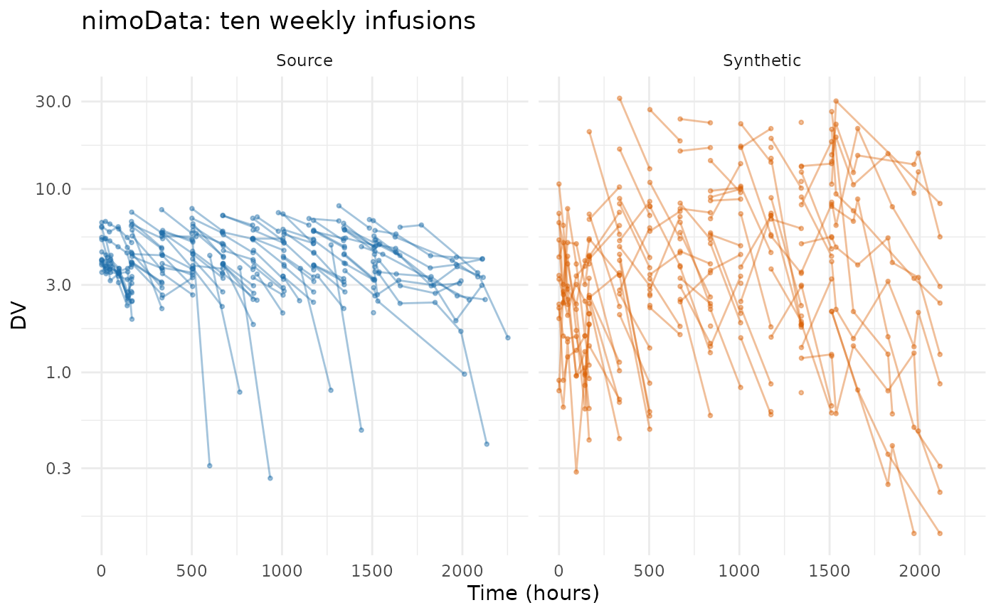

synpmx_scorecard_datatable(nimo_run$card, report = "minimal")

The generation screen warns that the simulated interquartile range is more than twice the source’s. The fit remains accepted: this is a spread warning, not a gross failure that triggers one-compartment fallback. D1 and the plot show the wider synthetic distribution. With only twelve subjects, the estimated population variability also has limited support; passing the checks does not make that variability precise.

nimoData is also the study that shows the other reading the fit has to make. It reports one negative concentration in 321 — what an assay returns for a sample near its limit — and a single row is not evidence that this endpoint reaches zero. Treating it as evidence would fit an additive residual to values whose median is 3, and the generated troughs would land on zero. It is substituted at half the smallest positive value the study reports, the fit says so as it happens, and the proportional residual stands.

pheno_sd: the grid has to be built, not declared

59 neonates on phenobarbital in routine care, with individualised dosing and sparse irregular sampling: 155 observations at 118 distinct times, about two and a half per baby. The concentration test fails here for the same reason it fails on nimoData — the doses are individualised rather than assigned, so nothing reads as dose-proportional.

data("pheno_sd", package = "nlmixr2data")
pheno_sd <- as.data.frame(pheno_sd)
pheno_flat <- pheno_sd
pheno_flat$NTIME <- pheno_flat$TIME   # a declaration this study cannot support
pheno_roles <- pmx_roles(
  id = "ID", time = "TIME", nominal_time = "NTIME", dv = "DV", amt = "AMT",
  evid = "EVID", mdv = "MDV", covariates = c("WT", "APGR")
)
synpmx_model_estimate(pheno_flat, pheno_roles, seed = 1)
#> Error:
#> ! No endpoint looks like a drug concentration: none is both absent before the
#> first dose and dose-proportional.
#>   Signals read: DV (post-dose yes, proportional no)
#>   Fix: Name the concentration with `endpoint_roles = c(pk = "...")`, or use
#>     `synpmx_avatar()` or `synpmx_pca()`, which fit no structural model. For
#>     a PD-only study, declare `endpoint_roles = c(pd = "...")`.

Name the endpoint and it fits. Nothing in the generator’s own requirements stops this study — and with NTIME set to TIME the output is still nearly empty.

pheno_flat_fit <- stored_fit("pheno-flat-model-fit.rds")
pheno_flat_synthetic <- synpmx_model_generate(pheno_flat_fit, seed = 707)
#> Warning: 92% of generated observations (23 of 25) fell below the emission floor and
#> were raised to it.
#>   A floor catching this much is a fitted model that does not describe the
#>   low end of the data, not an assay limit.
#>   Fix: Read `model_report()` before using this dataset.
c(distinct_times = length(unique(pheno_sd$TIME[pheno_sd$EVID == 0])),
  grid_cells = nrow(pheno_flat_fit$cells),
  source_obs_per_patient = round(sum(pheno_sd$EVID == 0) /
                                   length(unique(pheno_sd$ID)), 2),
  synthetic_obs_per_patient = round(
    sum(pheno_flat_synthetic$EVID == 0) /
      length(unique(pheno_flat_synthetic$ID)), 2))
#>            distinct_times                grid_cells    source_obs_per_patient 
#>                    118.00                      5.00                      2.63 
#> synthetic_obs_per_patient 
#>                      0.47

118 distinct recorded times become a handful of grid cells. A cell has to be reached by enough patients to be a visit rather than one baby’s afternoon, and one clock reading per patient clears that almost nowhere. The visit model then has almost no place to put an observation, so what comes back is a legal dataset in the source’s shape holding almost nothing — and the run says so on the way past, because most of what little was drawn landed under the emission floor, the lowest concentration the generator will write.

The grid this study does have

The ward gives phenobarbital on a twelve-hour cycle and reads a concentration about once a day. Neither is written in the file and both are things a reader of the study can say, which is exactly what nominal_time is for: the clock is what happened, the grid is what was meant to happen. Snapping the dose times to twelve hours and the sample times to the day is that statement, and it is two lines.

pheno_sd$NTIME <- ifelse(
  pheno_sd$EVID == 0,
  snap_to(pheno_sd$TIME, c(2, seq(24, 408, by = 24))),   # about one a day
  snap_to(pheno_sd$TIME, seq(0, 168, by = 12))           # the q12h cycle
)

pheno_run <- model_run("pheno_sd", pheno_sd, pheno_roles,
                       "pheno-model-fit.rds", seed = 707)
#> Warning: 10% of generated observations (17 of 164) fell below the emission floor and
#> were raised to it.
#>   A floor catching this much is a fitted model that does not describe the
#>   low end of the data, not an assay limit.
#>   Fix: Read `model_report()` before using this dataset.
pheno_run$fit
#> A fitted PMX model, from synpmx_model_estimate()
#> Everything below is an input to `synpmx_model_generate()`.
#> 
#>   candidates fitted  2 (2cmt_iv selected) 
#> 
#> Summarized from the source, not estimated
#>   cohort             59 patients in 1 arm(s)
#>                      all (59)
#>   dose changes       per planned cycle, pooled over arms: reduce 29%, skip
#>                      1%, stop early 10% (4 dose level(s))
#>   visit grid         1 endpoint(s) at 9 nominal time(s), 9 slot(s) in all
#>   visit attendance   share of scheduled slots attended, one rate per
#>                      endpoint: DV 28%
#>   covariates         WT lognormal, APGR lognormal, drawn once for the whole
#>                      study, independently of the profiles
#>   columns emitted    ID, TIME, NTIME, DV, AMT, EVID, MDV, WT, APGR
#> 
#> Values at the lower limit of what was observed
#>     DV                 5, no assay limit: half the lowest value several patients reached, rounded down
#> 
#> PK endpoint for the PopPK model
#>   DV                 declared through `endpoint_roles`
#>   route              both: too few distinct sampling times to place a peak
#>   sampling           median 1 distinct times after a dose, 0 after the
#>                      peak: sparse within-subject sampling
#> 
#> The PopPK model
#> 
#> Estimated by nlmixr2
#>   structural model   2cmt_iv 
#>   selected by        two-compartment model passed acceptance checks; lowest
#>                      AIC among accepted routes
#>   fitted on          all 59 patients with a concentration
#>   fixed effects      cl 0.006, v 0.8, q 0.6, v2 0.6 
#>   between-subject    cl 0.316, v 0.707, q 0.1, v2 0.245 (as SD on the log scale)
#>   residual error     proportional 0.1 
#>   time to fit        2 min 30 s
#>                        2cmt_iv                    52.4 s
#>                        2cmt_oral                  1 min 38 s
#>   whole call         2 min 30 s, against 2 min 30 s in the fitter
#> 
#> Privacy
#>   one patient's pull pass: largest: APGR SD on the log scale, 4.32 points;
#>                      `model_privacy_checks()` has every check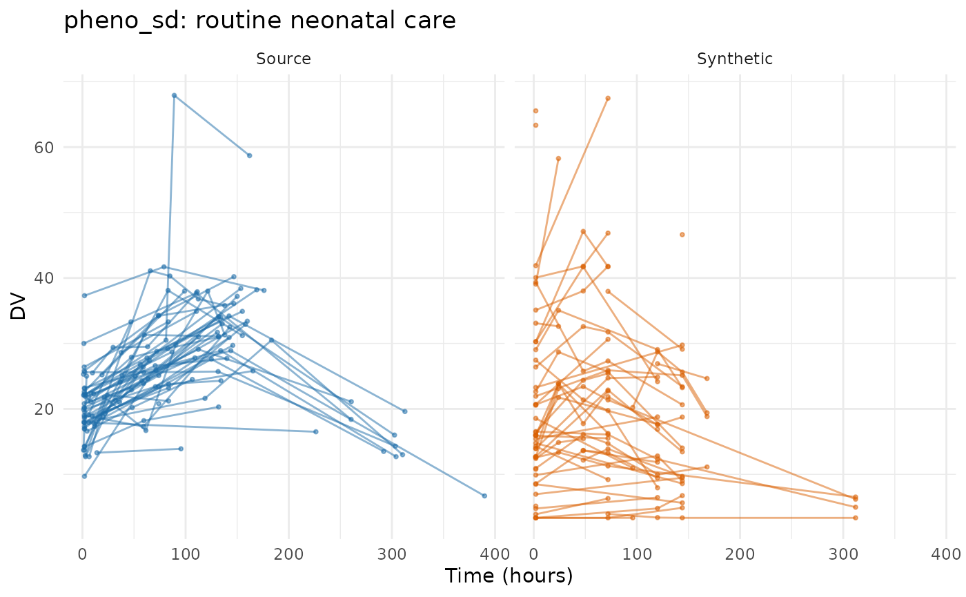

synpmx_scorecard_datatable(pheno_run$card, report = "minimal")

The fixed effects are the same either way, and that is the point worth holding on to: estimation reads the recorded clock and the recorded dosing history, so the grid never touches it. What the grid decides is the visit model, and the visit model is the whole of what the generated study has. With somewhere to put an observation, observations per patient come back.

This sparse design has no dose interval with enough observations for the usual starting-value calculation. Its starts are read from the cohort’s dose amounts and concentrations instead.

Passing acceptance checks does not establish a distribution phase. This study has sparse sampling within dose intervals. The fit report shows whether two compartments passed the checks or required fallback, but a numerically usable split between central and peripheral volumes does not establish that both volumes are identified by these observations.

What has not moved is the dosing: every baby in pheno_sd is dosed to their own weight and response, and the dosing model carries one planned schedule per arm, with one set of reduction, interruption and discontinuation rates for the study. The generated babies all follow the ward’s cycle rather than their own.

This is still the study to read before declaring a nominal grid, but the lesson is the opposite of a refusal: the generator will accept NTIME <- TIME and hand back what it implies, and the work of using it on a study like this is deciding what the protocol would have said. synpmx_pca() refuses the declaration outright; synpmx_avatar() derives a grid instead, and the AVATAR evaluation runs this study that way.

mixroute_sim: two routes, and a bioavailability that is known

Ninety patients dosed intravenously, subcutaneously, and both. This is the study 1cmt_mixed exists for, and because it is simulated the fit can be graded rather than merely read: the truth is a clearance of 2 L/day, a volume of 10 L, an absorption rate of 0.5 /day and a bioavailability of 0.7. The fitted parameters and generated profiles can be compared with that known truth. The default may accept two compartments even on this one-compartment study; the candidate table reports whether fallback was needed.

mixroute_roles <- pmx_roles(
  id = "ID", time = "TIME", nominal_time = "NTIME", dv = "DV", amt = "AMT",
  evid = "EVID", cmt = "CMT", adm = "ADM",
  routes = c("1" = "iv", "2" = "extravascular"),
  cens = "CENS", strata = "ARM", covariates = "WT"
)
mixroute_run <- model_run("mixroute_sim", mixroute_sim, mixroute_roles,
                          "mixroute-sim-model-fit.rds", seed = 808)
mixroute_run$fit
#> A fitted PMX model, from synpmx_model_estimate()
#> Everything below is an input to `synpmx_model_generate()`.
#> 
#>   candidates fitted  1 (2cmt_mixed selected) 
#> 
#> Summarized from the source, not estimated
#>   cohort             90 patients in 3 arm(s)
#>                      IV only (30)
#>                      SC only (30)
#>                      IV then SC (30)
#>   dose routes        iv and extravascular; given as a bolus
#>   dose changes       none
#>   visit grid         1 endpoint(s) at 17 nominal time(s), 17 slot(s) in all
#>   visit attendance   share of scheduled slots attended, one rate per
#>                      endpoint: DV 100%
#>   covariates         WT lognormal, drawn once for the whole study,
#>                      independently of the profiles
#>   columns emitted    ID, TIME, NTIME, DV, AMT, EVID, CMT, CENS, ADM, WT,
#>                      ARM
#> 
#> Values at the lower limit of what was observed
#>   Reported below the assay limit:
#>     DV                 3 of 1530 (0%) below 0.05 (the limit)
#> 
#> PK endpoint for the PopPK model
#>   DV                 inferred from the following data characteristics:
#>                        absent before the first dose
#>                        recorded in the compartment the doses go into
#>                        rises to one peak and comes back down within one
#>                          dose interval
#>   route              mixed: declared through `adm` and `routes`: iv and
#>                      extravascular doses in one study
#>   sampling           median 9 distinct times after a dose, 3 after the
#>                      peak: richer within-subject sampling
#> 
#> The PopPK model
#> 
#> Estimated by nlmixr2
#>   structural model   2cmt_mixed 
#>   selected by        two-compartment model passed acceptance checks
#>   fit checks         Warning: the optimizer stalled before convergence was
#>                      confirmed. Check that the synthetic data reasonably
#>                      reproduces the source data's patterns and
#>                      variability.; median checked against censoring bounds;
#>                      spread comparison omitted for censored observations
#>   fitted on          60 of 90 patients with a concentration, drawn in
#>                      proportion to the arms under `max_fit_subjects` = 60;
#>                      the dosing, visit and covariate models below read the
#>                      whole study
#>   fixed effects      cl 2, v 10, q 2, v2 0.1, ka 0.5, f 0.7 
#>   between-subject    cl 0.316, v 0.265, q 0.316, v2 0.283, ka 0.316 (as SD on the log scale)
#>   residual error     proportional 0.3 
#>   time to fit        33.8 s
#>   whole call         33.9 s, against 33.8 s in the fitter
#> 
#> Privacy
#>   one patient's pull pass: largest: DV: ka between-subject SD, 4.25 points;
#>                      `model_privacy_checks()` has every check

# The fit's estimates at full precision: the fingerprint carries them at one
# significant figure, which would grade the rounding rather than the fit.
full_precision <- function(fit) {
  estimated <- fit$pk_models[[1L]]$estimated
  (if (is.null(estimated)) fit$parameters else estimated)$fixed
}
truth <- c(cl = 2, v = 10, ka = 0.5, f = 0.7)
fitted <- full_precision(mixroute_run$fit)[names(truth)]
data.frame(truth = truth, fitted = round(fitted, 3),
           ratio = round(fitted / truth, 2))
#>    truth fitted ratio
#> cl   2.0  2.445  1.22
#> v   10.0 11.490  1.15
#> ka   0.5  0.515  1.03
#> f    0.7  0.737  1.05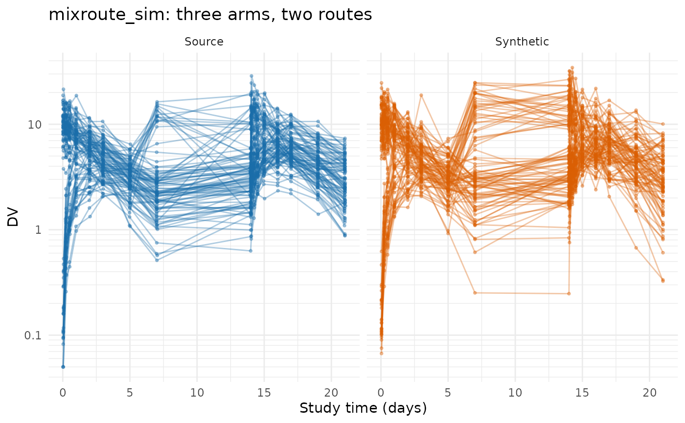

synpmx_scorecard_datatable(mixroute_run$card, report = "minimal")

The truth table compares estimated bioavailability with the value used to simulate this study. That comparison depends on fitting the two routes as one study. f is identifiable here because the same study doses both ways; on either arm alone it is confounded with clearance and volume and cannot be estimated at all. It is fitted as a fixed effect with no between-subject term, because a design with one dose each way identifies the contrast between the routes and not a distribution over it.

onc_sim: a slow endpoint, and a concentration sampled only at troughs

Two hundred patients, a year of daily everolimus, tumour size beside trough concentrations. Two things here defeat the parts of this generator that read a curve.

The baseline separates the endpoints. Tumour size is positive at the first dose and is classified as PD; the everolimus trough remains PK. The stored fit also declares the concentration explicitly, which gives the same assignment.

The concentration is sampled only at troughs. The starting values are a non-compartmental read of the median profile, which needs a peak and a terminal slope; a trough series has neither, and the absorption rate started two orders of magnitude from everolimus’s own. start_param states what is known about the compound instead, and the clearance and volume are still read off the curve.

onc_roles <- pmx_roles(
  id = "ID", time = "TIME", nominal_time = "NTIME", dv = "DV", amt = "AMT",
  evid = "EVID", cmt = "CMT", dvid = "NAME", addl = "ADDL", ii = "II",
  cens = "CENS", strata = "ARM", covariates = c("BSLD", "AGE", "SEX"),
  keep = "CROSSOVER"
)
onc_run <- model_run("onc_sim", onc_sim, onc_roles, "onc-sim-model-fit.rds",
                     seed = 808)
onc_run$fit
#> A fitted PMX model, from synpmx_model_estimate()
#> Everything below is an input to `synpmx_model_generate()`.
#> 
#>   candidates fitted  2 (2cmt_oral selected) 
#> 
#> Summarized from the source, not estimated
#>   cohort             200 patients in 2 arm(s)
#>                      Everolimus 10 mg (134)
#>                      Placebo (66)
#>   dose changes       per planned cycle, pooled over arms: reduce 0%, skip
#>                      5%, stop early 0% (2 dose level(s))
#>   visit grid         2 endpoint(s) at 24 nominal time(s), 30 slot(s) in all
#>   visit attendance   share of scheduled slots attended, one rate per
#>                      endpoint: Everolimus trough 65%, SLD 89%
#>   covariates         BSLD lognormal, AGE lognormal, SEX categorical, drawn
#>                      once for the whole study, independently of the
#>                      profiles
#>   columns emitted    ID, TIME, NTIME, DV, AMT, EVID, CMT, NAME, CENS, ADDL,
#>                      II, BSLD, AGE, SEX, ARM, CROSSOVER
#> 
#> Values at the lower limit of what was observed
#>   Reported below the assay limit:
#>     Everolimus trough  203 of 1167 (17%) below 1 (the limit)
#>     SLD                2, no assay limit: half the lowest value several patients reached, rounded down
#> 
#> Each non-PK continuous endpoint, fitted as constant, linear, or exponential
#>   SLD                linear
#>                        baseline         20
#>                        slope            -0.005
#>                        between-subject  0.3 (SD on the log baseline)
#>                        residual         additive 1
#>                        chosen on AIC from constant, linear, exponential
#> 
#> PK endpoint for the PopPK model
#>   Everolimus trough  declared through `endpoint_roles`
#>   route              both: too few distinct sampling times to place a peak
#>   sampling           median 1 distinct times after a dose, 0 after the
#>                      peak: sparse within-subject sampling
#> 
#> The PopPK model
#> 
#> Estimated by nlmixr2
#>   structural model   2cmt_oral 
#>   selected by        two-compartment model passed acceptance checks; lowest
#>                      AIC among accepted routes
#>   fit checks         median checked against censoring bounds; spread
#>                      comparison omitted for censored observations
#>   fitted on          60 of 200 patients with a concentration, drawn in
#>                      proportion to the arms under `max_fit_subjects` = 60;
#>                      the dosing, visit and covariate models below read the
#>                      whole study
#>   fixed effects      cl 0.4, v 0.6, q 0.01, v2 0.5, ka 3 
#>   between-subject    cl 0.447, v 0.0894, ka 0.173, q 0.0632, v2 0.141 (as SD on the log scale)
#>   starting values    ka 5 declared through `start_param`; the rest were
#>                      read off the cohort's median profile
#>   residual error     proportional 0.2 
#>   time to fit        35 min 36 s
#>                        2cmt_iv                    12 min 52 s
#>                        2cmt_oral                  22 min 44 s
#>   whole call         35 min 42 s, against 35 min 36 s in the fitter
#> 
#> Privacy
#>   one patient's pull pass: largest: SLD slope, 0.635 SE;
#>                      `model_privacy_checks()` has every check

The stored fit above was built with endpoint_roles = c(pk = "Everolimus trough") and start_param = c(ka = 5). Tumour size becomes the PD endpoint and is fitted a time course.

truth <- c(cl = 0.470, v = 0.850, ka = 5)
fitted <- full_precision(onc_run$fit)[names(truth)]
data.frame(truth = truth, fitted = round(fitted, 3),
           ratio = round(fitted / truth, 2))
#>    truth fitted ratio
#> cl  0.47  0.423  0.90
#> v   0.85  0.551  0.65
#> ka  5.00  3.402  0.68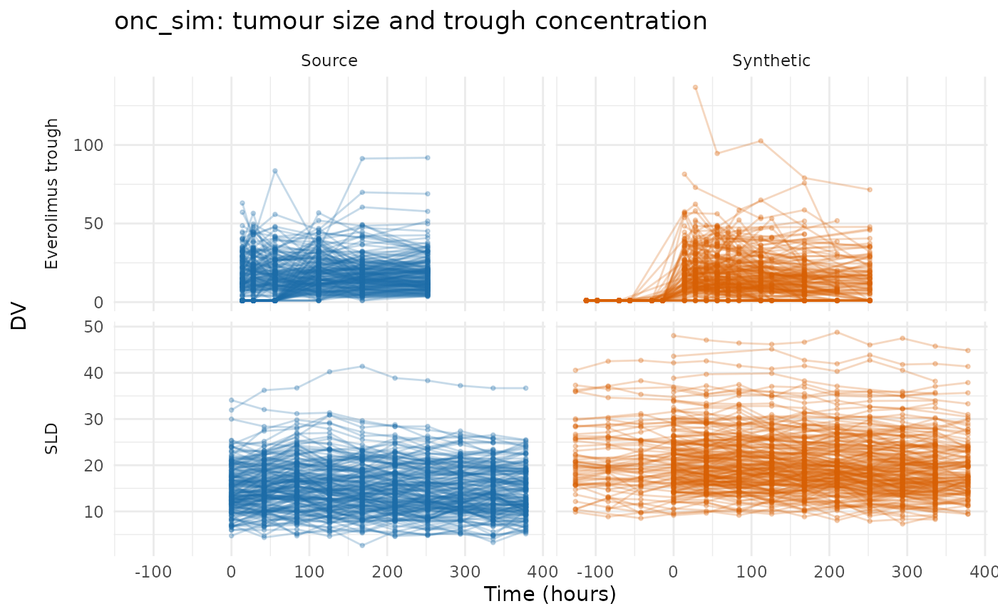

synpmx_scorecard_datatable(onc_run$card, report = "minimal")

Read the tumour endpoint against what it is: a PD time course here is a function of time with no exposure term and no dose term, pooled across arms unless pd_by_arm = TRUE. The source’s placebo and 10 mg arms diverge because the dose drives the tumour; the generated ones follow one shape. The dosing comes through as each arm’s planned schedule, changed at rates pooled over both arms, and the endpoint that responds to it does not respond at all; on this study that gap is the whole scientific content.

What the accepted fits held

inventory <- do.call(rbind, lapply(runs, function(entry) {
  fit <- entry$fit
  data.frame(
    Dataset = entry$label,
    Patients = length(unique(entry$source[[entry$roles$id]])),
    Model = if (is.null(fit$structural)) "PD only" else fit$structural,
    `Fixed effects` = if (is.null(fit$parameters)) "PD parameters shown above" else paste(names(fit$parameters$fixed),
                            signif(fit$parameters$fixed, 3),
                            collapse = ", "),
    # A proportional error reports a coefficient of variation and an additive
    # one a standard deviation, so the field is named by the kind.
    Residual = if (is.null(fit$parameters)) "PD residuals shown above" else paste(fit$parameters$residual$kind,
                     signif(if (is.null(fit$parameters$residual$cv))
                              fit$parameters$residual$sd else
                              fit$parameters$residual$cv, 3)),
    check.names = FALSE, stringsAsFactors = FALSE
  )
}))
knitr::kable(inventory, row.names = FALSE,
             caption = "What each fit carries out of its study.")

What each fit carries out of its study.
Dataset	Patients	Model	Fixed effects	Residual
case1_pkpd	180	2cmt_oral	cl 10, v 60, q 8, v2 200, ka 2	proportional 0.3
mad	60	2cmt_oral	cl 6, v 50, q 5, v2 100, ka 1	proportional 0.4
warfarin	32	2cmt_oral	cl 0.1, v 7, q 0.1, v2 2, ka 0.4	proportional 0.2
wbcSim	45	PD only	PD parameters shown above	PD residuals shown above
mavoglurant	120	2cmt_infusion	cl 0.04, v 0.1, q 0.05, v2 0.2	proportional 0.3
theo_md	12	2cmt_oral	cl 3, v 30, q 2, v2 4, ka 1	proportional 0.2
nimoData	12	2cmt_infusion	cl 0.06, v 40, q 0.1, v2 300	proportional 0.4
pheno_sd	59	2cmt_iv	cl 0.006, v 0.8, q 0.6, v2 0.6	proportional 0.1
mixroute_sim	90	2cmt_mixed	cl 2, v 10, q 2, v2 0.1, ka 0.5, f 0.7	proportional 0.3
onc_sim	200	2cmt_oral	cl 0.4, v 0.6, q 0.01, v2 0.5, ka 3	proportional 0.2

verdicts <- do.call(rbind, lapply(runs, function(entry) {
  card <- as.data.frame(entry$card)
  counts <- table(factor(card$verdict,
                         levels = c("pass", "review", "FAIL",
                                    "not applicable")))
  data.frame(Dataset = entry$label, as.list(counts),
             Failing = paste(card$check[card$verdict == "FAIL"],
                             collapse = ", "),
             check.names = FALSE, stringsAsFactors = FALSE)
}))
knitr::kable(verdicts, row.names = FALSE,
             caption = "Scorecard verdicts across the accepted runs.")

Scorecard verdicts across the accepted runs.
Dataset	pass	review	not applicable
case1_pkpd	14	2	5
mad	15	1	5
warfarin	15	1	5
wbcSim	13	3	5
mavoglurant	13	3	5
theo_md	15	1	5
nimoData	15	1	5
pheno_sd	13	3	5
mixroute_sim	15	1	5
onc_sim	14	2	5

The verdicts above report which checks pass, require review or fail on each accepted run. Rejected fits do not contribute a synthetic cohort to this table.

What is preserved, and what is not

Each accepted fit stores the schema, nominal grid, arm sizes, dose schedules and covariate summaries. The scorecards above assess their realized reproduction in the generated cohorts; B4b checks that measured values were not copied.

Not preserved, with the study that shows each:

Visit-to-visit measurement noise. Every profile is one structural model at a different parameter draw, so generated profiles are smoother than real ones. Visible on every dataset here.
Exposure-response. The PD shapes are fitted to the pooled observations with no exposure term, so a synthetic patient’s arm does not reach their response. mad is the worked case, and onc_sim shows why it matters for an exposure-driven tumour response.
When patients missed visits or responded, and differences between arms. Attendance is one rate per endpoint, a binary or ordinal endpoint one set of level frequencies (one per arm under pd_by_arm = TRUE), and the dose changes three rates pooled over the arms. A late visit few patients reached is drawn as often as an early visit of the same endpoint, a response does not change over the visits, and an arm whose patients dropped out, reduced or responded more often than the others’ takes the study’s average. onc_sim and mad are the worked cases.
Per-patient dose schedules, and multiple periods. One planned schedule per arm. mavoglurant is the worked case: occasions per patient fall from 1.65 to 1. pheno_sd is the other half of it — every neonate is dosed to their own weight and response, and the generated babies all follow the ward’s cycle.
A delayed decline followed by recovery. The PD-only wbcSim example has this response shape; the current PD time courses cannot reproduce it.
Anything the declared grid does not hold. The visit model can only place an observation where the grid has a cell enough patients reached, so a grid that describes nothing produces a study that holds nothing. pheno_sd declared as NTIME <- TIME is the worked case, and the fidelity rows are where it shows.
Spread, on a cohort of twelve. nimoData and theo_md are both twelve subjects, and D1 reads a synthetic spread away from the source’s on each: a covariance matrix estimated from twelve people and drawn from freely is not the spread of the twelve it came from.

Where to go next

vignette("pmxmodel-algorithm") — what each step of the generator does.
vignette("pmxmodel-demo") — one study end to end, with the fit inspected.
vignette("pmxmodel-fingerprint") — every quantity a fit carries out of a study.
Evaluating PCA on public data and Evaluating AVATAR on public data — the same eight studies through the other two generators.
Privacy protections in the PMX model generator — the privacy checks on each of these fits.

Andrew Stein