The synpmx data generation algorithms

What this package does

synpmx builds synthetic pharmacometric (PMX) datasets: dosing and measurement event tables with the same schema, event grammar, and rough behavior as a real study, so that data-assembly code, diagnostic plots, and model-run plumbing can be developed outside the restricted environment that holds the real data.

That narrow purpose is important. A generated dataset is not anonymous data and is not a formal proof that source subjects cannot be re-identified. It is also not suitable for estimation, model selection, inference, dose selection, or clinical decisions. The method aims for structural usefulness, not scientific equivalence.

Given that synthetic data is oven used as a way to protect privacy, this package offers several synthetic data generation functions that offer different privacy guarantees.

They fall into two groups, and the split is what to read this vignette by.

Generators that read the study. Three of them, each carrying something different out of the source. synpmx_model() estimates a population pharmacokinetic model and simulates from it. synpmx_pca() reduces each subject to principal-component scores and models the scores. synpmx_avatar() blends real neighbouring patients’ values. None makes a formal privacy claim, and the first two need a declared nominal-time column.

Generators that assert a model instead. Three more, which take a public structural model and, in two cases, spend a differential-privacy budget to correct it against the study.

All six run below on one dataset, in the order they carry less and less of the study out with them:

PMX model — estimate a population model and simulate from the parameters.
PCA — fit a basis of the observed profiles and draw new scores on it.
AVATAR blending [1, 2] — build each synthetic subject out of real subjects.
Prior only — read no data at all; simulate from a public model.
Calibration — simulate from a public model whose magnitude is corrected by a small, differentially private release.
Empirical — release a dense set of differentially private summaries and rebuild subjects from them.

The order is not a ranking. Modes 1 to 3 are the ones to use when the output stays inside the source data’s own controls; modes 5 and 6 are the ones that survive crossing a trust boundary, and the panels below show what that costs at a cohort this size.

“AVATAR” is a method name rather than an initialism, from the patient-centric avatarization literature in which each synthetic record is built from the local neighborhood of real records. The original method is due to Guillaudeux and colleagues [2]; Destere and colleagues benchmark a modified AVATAR against other synthesis algorithms for population PK [1]. This package implements an AVATAR-inspired adaptation for longitudinal event tables, not published AVATAR software.

This vignette stays at the level of what each mode does and when to use it. The full AVATAR algorithm, every step with its mathematics and edge cases, is in the AVATAR Algorithm article.

The example: theophylline

theo_md (from nlmixr2data) is a small public dataset — 12 subjects, seven daily 320 mg oral doses, one concentration endpoint. Twelve subjects is a deliberately hard case: it is typical of early-phase work and it is where the differences between these modes are most visible.

data("theo_md", package = "nlmixr2data")
theo_md <- as.data.frame(theo_md)
str(theo_md)
#> 'data.frame':    348 obs. of  7 variables:
#>  $ ID  : int  1 1 1 1 1 1 1 1 1 1 ...
#>  $ TIME: num  0 0 0.25 0.57 1.12 2.02 3.82 5.1 7.03 9.05 ...
#>  $ DV  : num  0 0.74 2.84 6.57 10.5 9.66 8.58 8.36 7.47 6.89 ...
#>  $ AMT : num  320 0 0 0 0 ...
#>  $ EVID: int  101 0 0 0 0 0 0 0 0 0 ...
#>  $ CMT : int  1 2 2 2 2 2 2 2 2 2 ...
#>  $ WT  : num  79.6 79.6 79.6 79.6 79.6 79.6 79.6 79.6 79.6 79.6 ...

Modes 1 and 2 place every value on the protocol’s grid and refuse without one, so the grid is written down first. The doses are exactly 24 h apart and the samples are not, so each sample is placed by the dose interval it falls in plus its time after that dose snapped to the planned times. Both lines below are statements about the protocol rather than derivations from the data, which is why they are in the document instead of inside a function.

snap_to <- function(x, grid) {
  grid[max.col(-abs(outer(x, grid, "-")), ties.method = "first")]
}
theo_doses <- seq(0, 144, by = 24)                           # the Q24H schedule
theo_samples <- c(0, 0.25, 0.5, 1, 2, 3, 4, 5, 7, 9, 12, 24) # planned samples

interval <- pmax(1L, findInterval(theo_md$TIME, theo_doses))
theo_md$NTIME <- ifelse(
  theo_md$EVID == 0,
  theo_doses[interval] +
    snap_to(theo_md$TIME - theo_doses[interval], theo_samples),
  theo_md$TIME
)
c(recorded = length(unique(theo_md$TIME[theo_md$EVID == 0])),
  nominal = length(unique(theo_md$NTIME[theo_md$EVID == 0])))
#> recorded  nominal 
#>      156       26

One declaration of what the columns mean serves all three data-reading generators.

theo_roles <- pmx_roles(
  id = "ID", time = "TIME", nominal_time = "NTIME", dv = "DV", amt = "AMT",
  evid = "EVID", cmt = "CMT", covariates = "WT"
)

Mode 1: PMX model

The most familiar route to a pharmacometrician: fit a population model to the study and simulate new subjects from the parameters. synpmx_model_estimate() works out which endpoint is the drug and what design produced it, fits the candidates that design admits and picks one on AIC; synpmx_model_generate() then reads the fit alone. No number a patient measured is in scope while the second call runs.

Twelve subjects is below the floor this generator sets for itself. It refuses under 20, because a covariance matrix fitted to fewer describes those subjects rather than a population, and the refusal is lifted here deliberately so that the mode can be shown on the same study as the other five.

model_fit <- synpmx_model_estimate(theo_md, theo_roles, seed = 1,
                                   min_subjects = 12L)   # below the floor

The chunk above is shown rather than run: fitting compiles a model, so this article reads a stored fit built by scripts/build-model-fits.R.

model_fit
#> A fitted PMX model, from synpmx_model_estimate()
#> 
#>   fitted on    12 patients, 1 arm(s)
#>   structural   1cmt_oral (chosen from 1 candidate(s) on AIC) 
#>   fixed        cl 2.858, v 34.2, ka 1.454 
#>   random on    cl, v, ka 
#>   pk endpoint  DV 
#> 
#>   These parameters are not estimates to report. They exist to make
#>   simulated profiles resemble the source study; the candidate set is too
#>   small and the covariate model too thin for any of them to answer a
#>   scientific question.
model_data <- synpmx_model_generate(model_fit, n_subjects = 12, seed = 11)

What leaves the study is the printed object and nothing else: a structural model, three fixed effects, a covariance matrix, a residual error, and a per-arm dosing and visit model. vignette("pmxmodel-fingerprint") is the itemised list, and the parameters are not estimates to report — the object prints that warning with itself.

Mode 2: PCA

Rather than asserting a curve shape, this generator measures one. Every subject’s profile becomes a vector on the nominal grid, a principal-component basis is fitted to those vectors, and new subjects are drawn as new scores on that basis. It reads the study without holding on to any subject’s values.

pca_summary <- synpmx_pca_summarize(theo_md, theo_roles, seed = 22)
pca_summary
#> A trial summary, from synpmx_pca_summarize()
#> 
#>   fitted on    12 patients, 1 arm(s): all (12) 
#>   endpoints    DV (26 visits modelled) 
#>   covariates   WT 
#>   components   2 (78% of variance) 
#>   dose term    factor 
#>   dosing       7 planned cycle(s) per arm | no reductions, interruptions or early stops 
#> 
#> synpmx_pca_generate() reads this object and nothing else. To look inside it:
#>   pca_report()      what it read out of the source data
#>   pca_dosing()      the planned dose schedule, per arm
#>   pca_dose_rates()  reduction, interruption and discontinuation
#>   pca_visits()      the probability of a visit, per arm
#>   pca_components()  the loadings, over time
pca_data <- synpmx_pca_generate(pca_summary, seed = 22)

Twelve subjects buy two components, holding 78% of the variance, as the summary above says. That is the visible cost: everything outside those two components, measurement noise from visit to visit included, is not reproduced, and the generated profiles are smoother than the source ones. vignette("pca-algorithm") is the specification and vignette("pca-fingerprint") itemises what the summary carries.

Mode 3: AVATAR blending

The least work of the three: synpmx_avatar() needs no grid, no model and no fit — only the data and a declaration of what the columns mean. For each synthetic subject it copies a real subject’s event skeleton, then fills the covariates and concentrations with a distance-weighted blend of that subject’s nearest compatible neighbors, plus noise.

avatar <- suppressWarnings(synpmx_avatar(theo_md, theo_roles, seed = 101))
#> synpmx_avatar(): no `dvid` declared, so every observation is treated as one endpoint.
#>   Correct for a single-endpoint study; declare `dvid` if this one has more.
#> SYNPMX ALERT: unique visit sets
#>   3 of 12 patients (25%) share every individual observation time with
#>   somebody, but the set of visits they have observations at is theirs alone
#>   -- a missed visit, a discontinuation, or follow-up that has not reached
#>   the later visits.
#>   Why it matters: no time grid can help here, however fine or coarse: a
#>     grid decides where the visits are, not which ones a patient turned up
#>     for.
#>   Fix: `min_pattern_share` already stops these sets being reused (see the
#>     run report). Screen the result with `flag_identifiable_subjects()` if
#>     it still matters.
validate_pmx(avatar, theo_roles)$valid
#> [1] TRUE

Nothing was elicited, nothing was assumed, and the output keeps the cohort size and every column named in theo_roles. synpmx_avatar() keeps only role-named columns and drops the rest — so a stray identifier cannot leak out of a real subject by being forgotten — and here every theo_md column has a role, so nothing is dropped. On a 12-subject dataset it also emits documented small-group fallback warnings (some event-pattern groups have only one usable donor); they are suppressed above and explained in the AVATAR Algorithm article.

What you cannot say about this output is that it is anonymous. It is assembled from real trajectories, so it inherits the source data’s handling obligations wherever it is used — a constraint on who may see it, not on which machine holds it.

What AVATAR does to obscure the source

AVATAR gives no formal guarantee, so the honest way to describe its protection is to list the mechanisms and say what each one does and does not cover. There are seven: five run by default, and two are measurements you run yourself.

1. Blending across donors. No synthetic subject’s measurements come from one real patient. Each avatar’s covariates and concentrations are a distance-weighted blend of at least k = 5 compatible real donors, and max_donor_weight = 0.50 caps any single donor at half the blend. This is what protects the values. It is also the only mechanism whose strength grows with cohort size, and it is why a source with fewer than k + 1 subjects triggers a loud alert rather than quietly producing near-copies.

2. Screening structurally extreme subjects (screen = TRUE). A source subject whose follow-up length or dose count exceeds twice the cohort’s 90th percentile is never used as an anchor, so no avatar inherits a conspicuous skeleton. Only those two axes are screened at generation, because dose magnitude is noisy under weight-based dosing and DV is blended rather than copied. After generation, flag_identifiable_subjects() screens four axes — follow-up time, dose count, dose magnitude, and peak DV — and remediate_identifiable_subjects() truncates, drops, or replaces what it finds. This catches subjects who are extreme.

3. Coarsening the visit grid, then re-refining it (coarsen_time = TRUE). Source times are collapsed onto a shared visit grid, and the per-visit deviations are pooled across the cohort and resampled independently onto each avatar. This is what protects the schedule, which blending does not touch: the event skeleton is copied verbatim from one anchor, and under actual recorded times almost every subject holds the only copy of their visit vector. The order is what makes it work — snapping is many-to-one and destroys the deviation, where perturbing the original time in place would leave it recoverable. The grid is the nominal_time role where one is declared, and inferred from the pooled times otherwise; the inferred case is best-effort and alerts loudly when it cannot collapse a subject. The cost is timing fidelity: an avatar’s deviation from nominal is drawn from the cohort rather than inherited.

4. Recomputing the dose from a blended covariate (automatic). When the dose is a fixed multiple of a baseline covariate within each assigned stratum — mg/kg, mg/m² — that multiplier is a protocol property the stratum shares, while the covariate is individual and already blended. So the multiplier is kept and the amount recomputed from the avatar’s own blended weight. Previously AMT was copied verbatim while covariates were blended, which both disclosed the anchor’s weight exactly and left every avatar violating its own protocol: a cohort dosed at exactly 5 mg/kg produced avatars from 4.4 to 5.3. Several dose levels are found by clustering the observed ratios, so a 1/2/3 mg/kg escalation is recognised without declaring the arm — and so is intra-patient escalation, where the level changes within a subject. Detection fails closed where the dose is unrelated to any covariate.

5. Sampling the attendance pattern (min_pattern_share, default 2). Once coarsening has put every subject on a shared visit grid, what remains of a schedule is which of those visits each subject attended. Every time is then shared, so no single visit is identifying — the combination of absences is, and a patient who missed weeks 2 and 3 is singled out by a fingerprint made of gaps. No grid fixes this at any resolution, because the grid decides where the visits are, not which ones a subject has. So the pattern is drawn from ones at least min_pattern_share subjects hold. Nobody leaves the cohort: a subject with a rare pattern still contributes measurements as a donor, only their distinctive absences stop being reproduced. Dose events are never sampled, since that could emit a regimen no protocol permits.

The default of 2 states exactly one thing: no synthetic patient carries a schedule unique to a real patient. Matching exact patterns alone would discard almost everything, because two patients who each missed one visit count as different patterns if they missed different visits. So the draw is two-stage: a shape first — how many visits were missed and whether the misses were terminal, contiguous, or scattered — then a real pattern of that shape if one clears the floor, and only otherwise a generated arrangement, which is rejected and redrawn if it lands on a pattern too rare to have been reusable. On warfarin that takes the loss from 12 patterns to 2. What is lost is resolution: how much missingness and what kind survive, which specific visits does not. Every run reports the figures, so the trade can be judged per study rather than assumed.

7. Measuring how close the values landed (compare_pmx_proximity(), manual). The measurement for mechanism 1. Blending protects the values, and this asks whether they landed too close to somebody real: each subject’s nearest neighbour is either in its own dataset or the other one, and under the ideal that is a coin flip. The null comes from splitting the source cohort in half and running the identical statistic, so small-sample artefacts cancel. Wide at pharmacometric cohort sizes — it catches a blatant leak, not a subtle one.

6. Checking for unique event skeletons (skeleton_uniqueness(), manual). Reports, per subject, how many others share its observation time vector, its observation count, and its event signature. Run it on the source before generating. It is a measurement, not a mitigation — what to do about what it finds is mechanism 2 or 3 depending on which class is exposed. Observation times are coarsening’s job; observation counts are the screen’s, because no grid can change a count and what survives coarsening is visits that are missing, for whatever reason; dose amount is neither’s, so weight-based dosing leaves a cohort unique on signature regardless — declaring dose_covariate in pmx_roles() is what stops the amount itself being one real patient’s, by rebuilding it from each avatar’s own blended covariate. Evaluating AVATAR on public data runs the before and after over every public dataset.

Two things none of these do. They do not bound what an adversary learns, which is what differential privacy provides and why the trust-boundary question below decides the mode rather than the mechanism list. And they do not defend against an attacker who already holds a suspected participant’s record and only wants to confirm membership — the mechanisms reduce the ways that attack succeeds without limiting how often it does.

Mode 4: prior only

The opposite extreme. Declare a public structural model and a public protocol, and simulate. No confidential data is read, so there is nothing to protect and no budget to spend: this is epsilon = 0, the strongest possible guarantee.

The typical parameter values must come from somewhere that is not the data — allometric scaling from preclinical work, a published model for the compound class, or the reasoning that set the starting dose.

Before reaching for this mode as a simulator, read what the built-in models can and cannot express. The catalogue is small on purpose: no covariate effects, no inter-occasion variability, no additive residual error, no ODE models. It produces a structurally correct dataset to develop code against, not a faithful rendering of an arbitrary pharmacometric model.

Others are working in parallel to develop a data simulation SKILL.md file to support development of such synthetic data. This work is important, but outside the scope of this package.

theo_model <- pmx_structural_model(
  pk = "1cmt_oral",
  typical = c(cl = 6, v = 35, ka = 1.5),          # deliberately imperfect
  source = "illustrative allometric scaling; never fitted to theo_md"
)
# theo_md samples richly on the first and last days and takes a single trough
# in between, which is the usual shape for a repeated-dose study. `sampling`
# takes one entry per dose so that can be said directly; a bare vector would
# apply the rich profile after all seven doses and oversample the study
# three-fold.
rich <- c(0, 0.25, 0.5, 1, 2, 4, 7, 9, 12, 24)
theo_design <- pmx_trial_design(
  dose_levels = 320, cohort_sizes = 12,
  sampling = list(rich, 0, NULL, NULL, NULL, NULL, rich),
  n_doses = 7, dose_interval = 24,
  source = "illustrative protocol"
)
theo_design
#> Public trial design
#>   doses: 320  (n = 12)
#>   dose times: 0, 24, 48, 72, 96, 120, 144
#>   sampling: 
#>     dose 1: 0, 0.25, 0.5, 1, 2, 4, 7, 9, 12, 24
#>     dose 2: 0
#>     dose 3: none
#>     dose 4: none
#>     dose 5: none
#>     dose 6: none
#>     dose 7: 0, 0.25, 0.5, 1, 2, 4, 7, 9, 12, 24
#>   source: illustrative protocol
prior_only <- synpmx_prior(theo_model, theo_design, n_subjects = 12, seed = 202)
head(prior_only, 3)
#>   ID      TIME NTIME       TAD OCC       DV AMT RATE EVID CMT DVID MDV CENS
#> 1  1 0.0000000  0.00 0.0000000   1       NA 320    0    1   1 <NA>   1    0
#> 2  1 0.0000000  0.00 0.0000000   1 0.000000   0    0    0   2   cp   0    0
#> 3  1 0.2447759  0.25 0.2447759   1 3.462932   0    0    0   2   cp   0    0
#>   DOSE
#> 1  320
#> 2  320
#> 3  320

The generated table uses the package’s own generated schema (pmx_generated_roles()), including nominal time, time after dose, and occasion columns. The clearance of 6 L/h assumed above is about twice the truth for theophylline, and the output shows it: concentrations run low. That is the honest cost of spending no budget — the data is exactly as good as the prior.

Mode 5: calibration

The middle path, and the recommended one when a formal guarantee is needed and the cohort is small. Both synpmx_calibrated() and synpmx_empirical() refuse to run until synpmx_enable_dp_engines() has been called once in the session — a deliberate speed bump.

synpmx_enable_dp_engines()
#> DP engines enabled for this session: the differentially private engines are complete and tested, but not under active development, carry known open findings, and have not been independently privacy-audited. See https://iamstein.github.io/synpmx/articles/synpmx-privacy.html for the trust-boundary decision rule and what a production release additionally needs.

Keep the public model’s shape, and spend a small privacy budget correcting only its magnitude.

Each subject is reduced to a bounded multiplicative correction of the model’s own prediction, clipped to a public prior range, and released with calibrated noise. Only two numbers leave the data: the correction and a noised subject count.

priors <- pmx_priors(pk = pmx_prior(c(1 / 4, 4), source = "scaling literature"))
pmx_preflight(priors, epsilon = 1, n_subjects = 12)
#> Pre-flight: d = 2, epsilon = 1, N = 12  ->  f = 0.167
#>  quantity prior_fold         f expected_fold_error
#>        pk         16 0.1666667            1.587401
#> 
#> Verdict: worthwhile
#> The release meaningfully narrows the prior.

pmx_preflight() costs nothing and reads no data: it answers “is this release worth its budget?” before any budget is spent.

calibrated_data <- synpmx_calibrated(
  data = theo_md, roles = theo_roles, model = theo_model,
  design = theo_design, priors = priors, epsilon = 1, seed = 303,
  backend = "public", public_source = TRUE   # theo_md is public; no DP claim
)

The correction pulled the assumed clearance toward the data. The release that produced this dataset travels with it, so the accounting is always at hand:

attr(calibrated_data, "synpmx_release")
#> Calibrated structural model (v3)
#>   released subject count: 12
#>   pk correction: 0.669x
#>   corrected typical: cl=4.01, v=35, ka=1.5
#>   epsilon: 1  (formal DP: FALSE)
#>   f = 0.167 (worthwhile)

Generation from that release is post-processing, so further datasets cost nothing. Draw them with synpmx_generate() rather than by calling synpmx_calibrated() again — a second fit would spend the budget a second time.

another <- synpmx_generate(calibrated_data, seed = 304)   # spends nothing

calibrated <- synpmx_calibrated(
  data = confidential, roles = theo_roles, model = theo_model,
  design = theo_design, priors = priors, epsilon = 1,
  backend = "opendp"
)

dp_backend_status()
#>   backend available version production
#> 1  OpenDP      TRUE  0.15.1       TRUE

At 12 subjects a genuine DP release of this correction is noisy enough that it is often censored at the prior boundary — the package warns when that happens, because the generated data then reflects the prior, not the study. The privacy article covers when the release is worth making.

Mode 6: empirical

The general-purpose private engine. Rather than asserting the curve shape, it measures it: it releases noised summaries for the subject count, event and regimen structure, observation timing, endpoint trajectories, baseline covariates, and censoring, then rebuilds subjects from those summaries. This buys realism that the public model does not contain, and pays for it by splitting one epsilon across many released quantities.

It also needs the most declaration: every clipping range, contribution limit, and budget share is an explicit public input.

empirical_data <- synpmx_empirical(
  data = theo_md, roles = theo_roles,
  endpoints = list(cp = pmx_endpoint(
    alignment = "dose_relative", transform = "log", shape = "occasion", cmt = 2
  )),
  epsilon = 5, delta = 0,
  bounds = pmx_bounds(
    time = c(0, 170), endpoints = list(cp = c(0, 30)), amt = c(0, 500),
    covariates = list(WT = c(40, 130))
  ),
  public_design = pmx_public_design(
    pmx_schema(theo_md), dose_evid = 101, dose_cmt = 1
  ),
  contribution_limits = pmx_contribution_limits(40, 8, 8, 30, 11),
  budget_allocation = pmx_budget_allocation(
    subject_count = 0.10, event = 0.15, timing = 0.15,
    covariates = 0.10, endpoints = 0.50, censoring = 0
  ),
  seed = 404,
  backend = "public", public_source = TRUE   # theo_md is public; no DP claim
)
privacy_report(empirical_data)
#> No DP claim: the input was explicitly asserted to be a public fixture.
#> Privacy unit: one subject's complete bounded longitudinal contribution
#> Adjacency: add-or-remove one complete subject
#> Backend: public-fixture 0.0.0.9000
#> Illustrative query allocation (not a DP accounting claim): epsilon = 5, delta = 0
#> No privacy guarantee is asserted for this public-source fixture model.

Note the requested epsilon = 5, five times the calibrated fit’s budget, for a worse result at this cohort size. That is not a bug: the same budget is being split six ways over dozens of released coordinates. This engine earns its keep on large pooled datasets, not on twelve subjects.

The six side by side

Every generated dataset above holds the same study in a different way. Pulled into one frame, they can be read against the source and against each other.

generated_roles <- pmx_generated_roles()
all_observations <- rbind(
  observations(theo_md, theo_roles, "Source"),
  observations(model_data, theo_roles, "1. PMX model"),
  observations(pca_data, theo_roles, "2. PCA"),
  observations(avatar, theo_roles, "3. AVATAR"),
  observations(prior_only, generated_roles, "4. Prior only"),
  observations(calibrated_data, generated_roles, "5. Calibration"),
  # The empirical engine restores the source schema, so it uses source roles.
  observations(empirical_data, theo_roles, "6. Empirical")
)
all_observations$method <- factor(all_observations$method,
                                  levels = unique(all_observations$method))
summaries <- do.call(rbind, lapply(
  split(all_observations$dv, all_observations$method),
  function(dv) {
    data.frame(
      n_observations = length(dv),
      median = stats::median(dv),
      p10 = stats::quantile(dv, 0.10, names = FALSE),
      p90 = stats::quantile(dv, 0.90, names = FALSE)
    )
  }
))
knitr::kable(
  summaries, digits = 2,
  caption = "Observed concentrations by generation mode"
)

Observed concentrations by generation mode
	n_observations	median	p10	p90
Source	264	5.74	1.25	9.30
1. PMX model	258	5.81	1.52	10.54
2. PCA	261	5.95	1.31	9.30
3. AVATAR	264	5.21	1.21	8.33
4. Prior only	240	3.16	0.28	6.43
5. Calibration	240	4.05	0.36	7.54
6. Empirical	264	4.43	0.43	11.96

The source panel first, then the six generated datasets in order. Each line is one subject’s concentration profile over the seven daily doses.

ggplot2::ggplot(
  all_observations,
  ggplot2::aes(time, dv, group = subject)
) +
  ggplot2::geom_line(alpha = 0.4, colour = "#1B6CA8") +
  ggplot2::geom_point(alpha = 0.5, size = 0.7, colour = "#1B6CA8") +
  ggplot2::facet_wrap(~ method, ncol = 3) +
  ggplot2::labs(
    x = "Study time (hours)", y = "Concentration",
    title = "One study, six generation modes"
  ) +
  ggplot2::theme_minimal()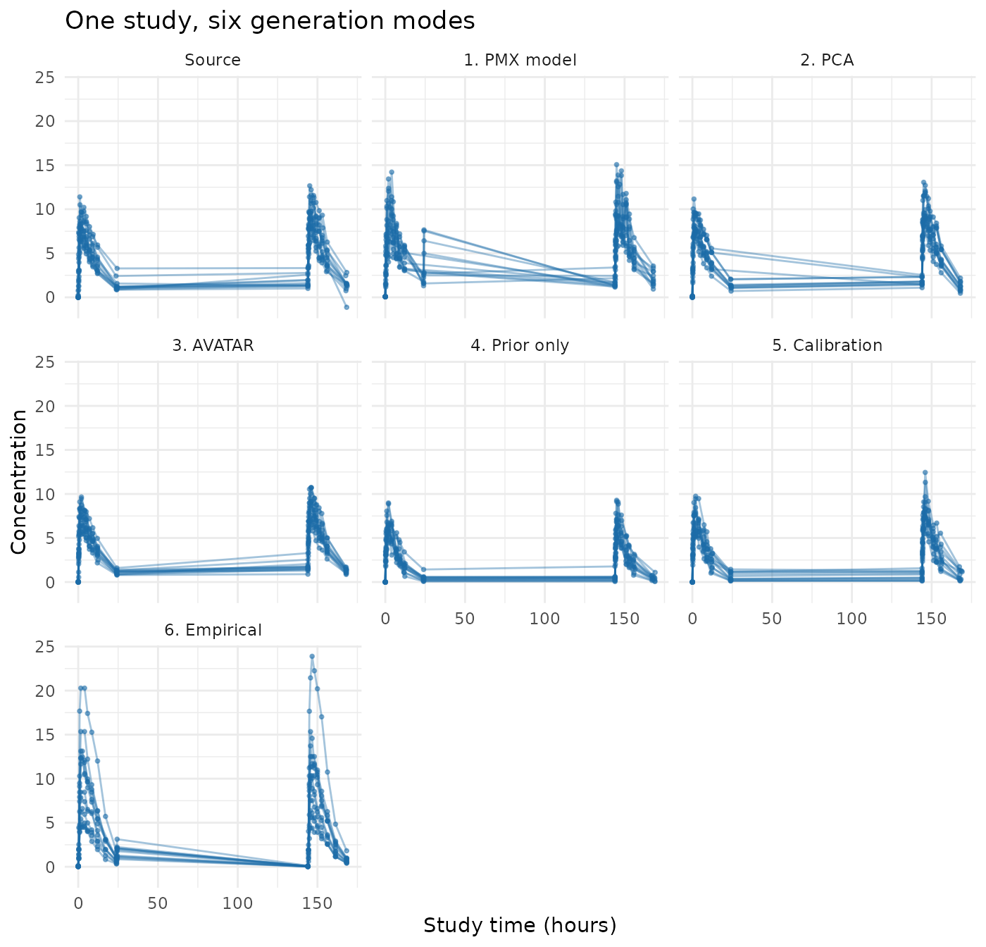

The table is the quickest read. The three data-reading modes land on the source’s concentrations — medians of 6.01, 5.95 and 5.21 against 5.74, and tenth and ninetieth percentiles within a few tenths — while the three public-model modes do not: 3.16, 4.05 and 4.43. That gap is the whole subject of this article.

Among the first three, mode 1 draws every profile from one structural model at a different parameter draw, so its profiles are the smoothest here and a real profile’s visit-to-visit wobble is absent. Mode 2 takes its shape from the observed profiles instead, and smooths within the two components twelve subjects buy. Mode 3 tracks the source most closely, because it is made of it.

Modes 4 to 6 are where the level goes. The prior-only data has the right structure and a clearance assumed about twice too fast, which is exactly the cost of reading nothing: its median concentration is 3.16 against the source’s 5.74. Calibration spends two numbers of budget pulling that level back toward the study, and gets to 4.05. The empirical engine, at five times the budget, does not do better in any way that matters: its median is 4.43, and its spread runs from a tenth percentile of 0.43 to a ninetieth of 11.96, against 1.25 and 9.30 in the source. It is not a study a pharmacometrician would work with.

The same six against the source, as distributions rather than profiles: the concentrations they generated, and the baseline weights they carried.

# One long frame of every value each mode produced, so concentration and weight
# can be drawn on the same panel row. A mode that carries no weight column --
# the public-model modes declare no covariates -- simply has no rows here.
weights <- function(data, roles, label) {
  covariate <- if ("WT" %in% names(data)) "WT" else NULL
  if (is.null(covariate)) return(NULL)
  first <- !duplicated(data[[roles$id]])
  data.frame(method = label, variable = "Baseline weight (kg)",
             value = as.numeric(data[[covariate]][first]),
             stringsAsFactors = FALSE)
}
distributions <- rbind(
  data.frame(method = all_observations$method,
             variable = "Concentration", value = all_observations$dv,
             stringsAsFactors = FALSE),
  weights(theo_md, theo_roles, "Source"),
  weights(model_data, theo_roles, "1. PMX model"),
  weights(pca_data, theo_roles, "2. PCA"),
  weights(avatar, theo_roles, "3. AVATAR"),
  weights(prior_only, generated_roles, "4. Prior only"),
  weights(calibrated_data, generated_roles, "5. Calibration"),
  weights(empirical_data, theo_roles, "6. Empirical")
)
distributions$method <- factor(distributions$method,
                               levels = levels(all_observations$method))

ggplot2::ggplot(distributions,
                ggplot2::aes(value, colour = method, linetype = method)) +
  ggplot2::stat_ecdf(linewidth = 0.6) +
  ggplot2::facet_wrap(~ variable, scales = "free_x") +
  ggplot2::scale_colour_manual(
    values = c("Source" = "#111111", "1. PMX model" = "#1B6CA8",
               "2. PCA" = "#2E8B57", "3. AVATAR" = "#D95F02",
               "4. Prior only" = "#7570B3", "5. Calibration" = "#A6761D",
               "6. Empirical" = "#B00020")
  ) +
  ggplot2::scale_linetype_manual(
    values = c("Source" = "solid", "1. PMX model" = "dashed",
               "2. PCA" = "dashed", "3. AVATAR" = "dashed",
               "4. Prior only" = "dotted", "5. Calibration" = "dotted",
               "6. Empirical" = "dotted")
  ) +
  ggplot2::labs(x = NULL, y = "Cumulative fraction", colour = NULL,
                linetype = NULL,
                title = "Observed concentrations and baseline weights, by mode") +
  ggplot2::theme_minimal() +
  ggplot2::theme(legend.position = "top")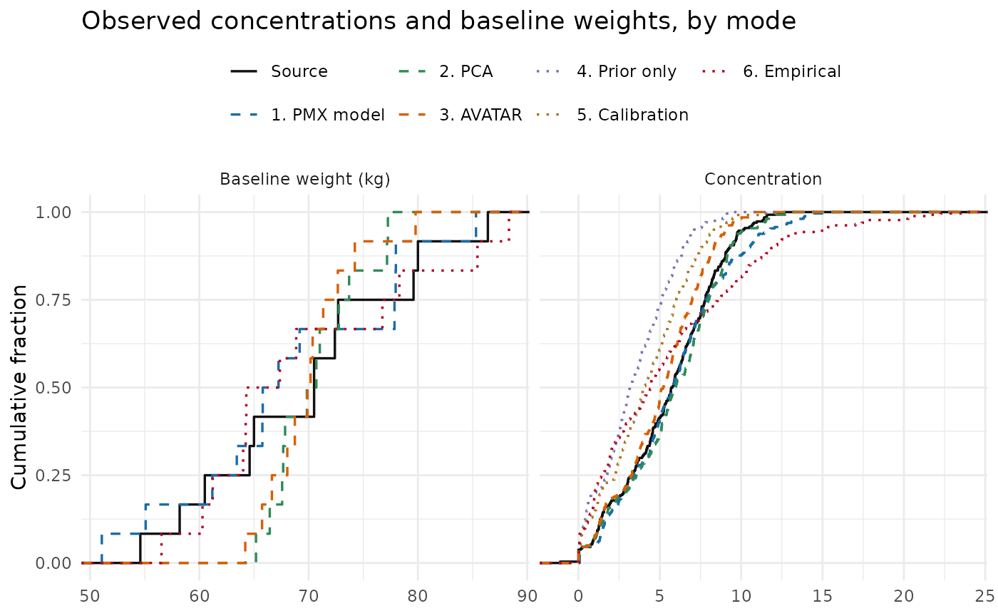

Read the concentration panel by how far each curve sits from the black one, and the weight panel by whether a mode has a curve there at all: the two public-model modes declare no covariates, so they generate no weights, and a covariate that is not declared is a column the output does not have.

Choosing a mode

Mode	Function	Output built from	Guarantee	Cohort size	Elicitation needed
1. PMX model	synpmx_model()	A population model fitted to the study, simulated forward	None; governance only	~20 and up	None, but a nominal grid is required
2. PCA	synpmx_pca()	A component basis of the observed profiles, and new scores on it	None; governance only	Any, from ~5, per arm	None, but a nominal grid is required
3. AVATAR blending	synpmx_avatar()	Real subject templates and blended real trajectories	None; governance only	Any, from ~5	None
4. Prior only	synpmx_prior()	A public model and protocol only	epsilon = 0 (no data read)	Any (data-independent)	Structural model + protocol
5. Calibration	synpmx_calibrated()	A public model, magnitude corrected by 2 private releases	(epsilon, delta) DP	~20 and up	Model, protocol, prior ranges
6. Empirical	synpmx_empirical()	Dozens of noised population summaries	(epsilon, delta) DP	~200 and up	Endpoints, bounds, limits, budget split

Where each mode belongs:

Environment	Appropriate modes	Why
Inside the validated environment holding the source data; you are the only consumer	PMX model, PCA or AVATAR	Access control and governance already bound the risk. A formal guarantee defends against an adversary who cannot reach the output, so it buys nothing and costs utility.
Shared with a partner, vendor, or contract research organization (CRO)	Calibration or Empirical, with an approved epsilon	The output leaves your controls. A contract is not a mathematical bound; DP is what survives a determined recipient.
Published, posted to a repository, or shipped inside a package or teaching material	Prior only, or Calibration with a small approved epsilon	Anyone may inspect it, forever, alongside side information you cannot anticipate. Prior-only data reads no patient record at all and is the safest thing to publish.
Software testing where only schema and event grammar matter	Prior only	Fidelity is irrelevant; a data-independent generator removes the question entirely.

Two rules of thumb behind the table:

The trust boundary decides the level of privacy needed. Ask whether the generated data can reach anyone the source data could not. A workstation under the same access controls reaches no one new. If no one new, AVATAR is more useful and its lack of a formal guarantee costs nothing. If someone new, only an accounted release holds up.
The cohort size decides which differential privacy mode is usable. Epsilon buys accuracy in proportion to the number of subjects and in inverse proportion to how many quantities you release. At 12 subjects, releasing two numbers can work and releasing fifty cannot.

Epsilon and delta are governance decisions, not defaults. For anything public facing they should be set and justified by whoever owns the data, and recorded: every fit carries a release ledger, and privacy_report() prints the realized accounting.

Why AVATAR is the default

Novartis’s synadam generates synthetic ADaM (Analysis Data Model) datasets by resampling each column marginally from the real data: a uniform draw over the observed range for continuous columns, a proportional resample for categorical ones, with no differential privacy. It preserves each column’s marginal support and relies on governance rather than a mathematical guarantee. That is standard, accepted practice.

AVATAR blending is the same governance-based idea applied at a different granularity: it resamples and blends whole subject trajectories rather than individual columns, because a pharmacometric endpoint is a correlated time-course that would be destroyed by independent per-column resampling. If synadam’s privacy model is acceptable for its use, AVATAR’s is acceptable for the same use — output kept under the source data’s own access controls, reaching no one the source data could not.

One caveat follows from the difference in granularity. A resampled covariate value (a weight of 72 kg) is weakly identifying because many people share it. A resampled subject trajectory is more strongly identifying because a full sampling-and-response pattern is more nearly unique. Blending several donors, adding noise, and removing outlying patients mitigates this, but not formally. AVATAR therefore depends on the governance context somewhat more than synadam’s column resampling does.

What the public-model modes replace

Modes 4, 5, and 6 do not read the study’s profiles at all. They replace the AVATAR pipeline entirely: there is no anchor subject, no donor neighborhood, and no event template. The trial structure comes from a declared public protocol (pmx_trial_design() or pmx_public_design()) rather than from a source subject’s rows.

Both differentially private engines are aggregate-based: no source subject’s rows, template, or trajectory reaches the output. They read the confidential data only through per-subject contributions clipped to publicly declared ranges, release those aggregates with calibrated noise, and generate from the noised numbers alone. They differ in what supplies the curve shape.

synpmx_calibrated() takes shape from a public structural model — a closed-form one-compartment or two-compartment PK model, evaluated analytically rather than by solving ordinary differential equations (ODEs) — and spends budget only on correcting its magnitude. The supported PK shapes are "1cmt_iv", "1cmt_oral", "1cmt_infusion", "2cmt_iv", and "2cmt_oral". Optional PD shapes are "constant", "linear", and "exponential", with no exposure dependence. Between-subject variability (iiv) and residual error (residual_cv) are public assumptions and consume no budget.

Because only a handful of numbers are released (d = 2 for a single PK correction plus the count), the noise per released quantity stays small, which is why this engine remains usable at 20 to 60 subjects. The tradeoff is that everything not calibrated is asserted: curve shape, variability, and residual error come from the public model, so the output is only as realistic as that model. It cannot reveal a structural feature the model does not contain.

synpmx_empirical() instead reconstructs shape from a denser set of noised summaries. It asserts less — trajectory shape is measured rather than assumed — but it releases far more numbers, so the same epsilon is split many ways. Utility therefore collapses below a few hundred subjects.

The built-in models are illustrative, and deliberately so

It is worth being blunt about the ceiling here, because the phrase “structural model” invites an expectation this package does not meet. The model catalogue is small and fixed:

	Supported
PK	`1cmt_iv`, `1cmt_oral`, `1cmt_infusion`, `2cmt_iv`, `2cmt_oral` — closed form, no ODEs
PD	`constant`, `linear`, `exponential`, with no exposure dependence
Variability	Lognormal between-subject variability on the typical parameters
Residual error	Proportional only

And that is the whole of it. There are no covariate–parameter relationships (no allometric exponent on clearance, no sex or biomarker effect), no inter-occasion variability, no additive or combined residual error, no absorption lag or transit compartments, no enzyme induction or time-varying parameters, no exposure-driven PD, and no user-supplied ODE model. Declared covariates appear in the output as columns, but nothing links them to the concentrations beside them.

This is a scope decision rather than a gap waiting to be filled. The space of pharmacometric models is effectively unbounded, and every study wants something idiosyncratic; a package that chased that would slowly become a worse rxode2, which already does the job properly. What the built-in models are for is narrow and useful: giving the DP engines a public backbone whose magnitude can be corrected under a budget, and producing structurally correct event tables to develop pipeline code against.

So if your question is “does my code handle this dataset shape?”, these modes are the right tool. If it is “what would this study look like under my model?”, write that model in rxode2 and simulate it there — that is the right tool, and an LLM is a capable assistant for producing the model code.

Where to go next

Evaluating AVATAR on public data — synpmx_avatar() run across eight public datasets, with the structural checks and the masking accounting for each.
Privacy — what differential privacy guarantees, what it does not, the trust-boundary decision rule, and how epsilon trades against utility.
The AVATAR Algorithm — the default generator step by step, and the six masking mechanisms.
The PCA Algorithm and its demo — the second data-reading generator, which fits a basis of the subject profiles rather than blending them.
The PMX Model Algorithm and its demo — the third, which estimates a linear population pharmacokinetic model and simulates from it. It is the only generator whose dose reductions reach the concentrations.
Model elicitation and data elicitation — how to produce the public model and protocol that modes 4 to 6 need.
Feasibility by cohort size — the measured evidence for what each private mode can deliver at your N.

References

Destere A, Lombardi R, Labriffe M, et al. Can synthetic data overcome the privacy and fidelity bottleneck in Pharmacometrics? A comparative benchmark using a daptomycin population pharmacokinetic model. medRxiv preprint, posted June 2, 2026. doi: 10.64898/2026.05.30.26354512.
Guillaudeux M, Rousseau O, Petot J, et al. Patient-centric synthetic data generation, no reason to risk re-identification in biomedical data analysis. npj Digital Medicine. 2023;6. doi: 10.1038/s41746-023-00771-5.

Andrew Stein