One case worked end to end: a synthetic pyrazinamide dataset, 1200 mg orally once daily for two weeks, sampled on day 14. Every number and every choice is shown, including the ones the generator cannot represent.
synpmx_prior() reads no data at all. It
takes a public structural model and a trial design and simulates from
those alone, so there is no data argument to supply and
nothing here needs a privacy argument. See Privacy
for where this sits among the method families.
The cardinal rule for this mode: every number below must come from
somewhere that is not the study being simulated. The values
used here are literature and protocol values for pyrazinamide, recorded
in each object’s source field. Fit a model to a real study
and paste its estimates in here and the real data reaches the output
through the parameters, making the “nothing was read” claim false.
synpmx_prior() cannot detect that, so the discipline is
yours to keep.
Read the last section before using the output. Three parts of the specification below cannot be expressed, and none of them fails loudly.
The specification
| Quantity | Value |
|---|---|
| Structural model | 1-compartment oral, first-order absorption and elimination |
| Ka | 1.31 h-1 |
| CL/F | 3.52 L/h |
| V/F | 28.57 L |
| IIV (log-SD) | Ka 0.620, CL 0.174, V 0.181 |
| IOV (log-SD) | V 0.117 |
| Residual error | proportional 0.22, additive SD 2.41 mg/L |
| WT, CD38, GENDER | not generated — see the last section |
| Regimen | 1200 mg orally once daily |
| Sampling | after 2 weeks of dosing, at 0.3, 0.9, 2.2, 4.5, 8 h post dose |
Choices the specification does not give, made here and flagged so they are easy to change:
N_SUBJECTS <- 60          # cohort size
SEED       <- 20260728    # reproducibility seed
LLOQ       <- 0.2         # mg/L, a typical HPLC assay limit for pyrazinamide
DROPOUT    <- 0           # no discontinuation modelled
N_DOSES    <- 14          # "2 weeks of dosing" at once daily
One unit conversion
pmx_structural_model(iiv = ) takes a
CV, while the specification gives
log-SD. These are different parameterisations of the
same lognormal, so the values are converted rather than pasted:
CV = sqrt(exp(omega^2) - 1).
omega_to_cv <- function(omega) sqrt(exp(omega^2) - 1)

iiv_log_sd <- c(ka = 0.620, cl = 0.174, v = 0.181)
iiv_cv     <- omega_to_cv(iiv_log_sd)
knitr::kable(
  data.frame(parameter = names(iiv_log_sd),
             log_sd = iiv_log_sd, cv = round(iiv_cv, 4)),
  row.names = FALSE, caption = "IIV: specification (log-SD) to package (CV)"
)| parameter | log_sd | cv |
|---|---|---|
| ka | 0.620 | 0.6846 |
| cl | 0.174 | 0.1753 |
| v | 0.181 | 0.1825 |
The public inputs
pza_model <- pmx_structural_model(
  pk      = "1cmt_oral",
  typical = c(cl = 3.52, v = 28.57, ka = 1.31),
  iiv     = iiv_cv,
  residual_cv = 0.22,
  source  = paste(
    "Published pyrazinamide population PK parameters; never fitted to the",
    "study being simulated."
  )
)
pza_model
#> Public structural model
#>   PK: 1cmt_oral
#>   PD: none
#>   typical: cl=3.52, v=28.6, ka=1.31
#>   source: Published pyrazinamide population PK parameters; never fitted to the study being simulated.
Sampling is requested only after two weeks of dosing, so thirteen
doses carry no samples and the fourteenth carries the full profile.
sampling takes one entry per dose, and NULL
means “no samples after this one”.
post_dose <- c(0.3, 0.9, 2.2, 4.5, 8)

pza_design <- pmx_trial_design(
  dose_levels   = 1200,
  cohort_sizes  = N_SUBJECTS,
  sampling      = c(rep(list(NULL), N_DOSES - 1L), list(post_dose)),
  n_doses       = N_DOSES,
  dose_interval = 24,
  source        = "Protocol: 1200 mg orally once daily for 2 weeks."
)
pza_design
#> Public trial design
#>   doses: 1200  (n = 60)
#>   dose times: 0, 24, 48, 72, 96, 120, 144, 168, 192, 216, 240, 264, 288, 312
#>   sampling:
#>     dose 1: none
#>     dose 2: none
#>     dose 3: none
#>     dose 4: none
#>     dose 5: none
#>     dose 6: none
#>     dose 7: none
#>     dose 8: none
#>     dose 9: none
#>     dose 10: none
#>     dose 11: none
#>     dose 12: none
#>     dose 13: none
#>     dose 14: 0.3, 0.9, 2.2, 4.5, 8
#>   source: Protocol: 1200 mg orally once daily for 2 weeks.
Naming the output columns
Every generator in the package takes a pmx_roles()
declaration and writes its output under those column names. The three
that read a study take it as a description of what they are reading;
this one reads nothing, so the same object does the opposite job here
and says which schema to generate into. Pass the roles of the study this
data has to stand in for, and the output drops straight into code
written against it.
pza_roles <- pmx_roles(
  id = "USUBJID", time = "TIME", nominal_time = "NTIME", tad = "TAD",
  occasion = "OCC", dv = "DV", amt = "AMT", evid = "EVID", cmt = "CMT",
  mdv = "MDV", cens = "CENS"
)
A role left undeclared gets no column, which is why there is no
RATE or DOSE below.
pmx_generated_roles() is the default and names every column
the generator can produce.
Generate
pza <- synpmx_prior(
  pza_model, pza_design, pza_roles,
  n_subjects = N_SUBJECTS, seed = SEED,
  dropout = DROPOUT, lloq = LLOQ
)

str(pza)
#> 'data.frame':    1140 obs. of  11 variables:
#>  $ USUBJID: int  1 1 1 1 1 1 1 1 1 1 ...
#>  $ TIME   : num  0 24 48 72 96 120 144 168 192 216 ...
#>  $ NTIME  : num  0 24 48 72 96 120 144 168 192 216 ...
#>  $ TAD    : num  0 0 0 0 0 0 0 0 0 0 ...
#>  $ OCC    : int  1 2 3 4 5 6 7 8 9 10 ...
#>  $ DV     : num  NA NA NA NA NA NA NA NA NA NA ...
#>  $ AMT    : num  1200 1200 1200 1200 1200 1200 1200 1200 1200 1200 ...
#>  $ EVID   : int  1 1 1 1 1 1 1 1 1 1 ...
#>  $ CMT    : int  1 1 1 1 1 1 1 1 1 1 ...
#>  $ MDV    : int  1 1 1 1 1 1 1 1 1 1 ...
#>  $ CENS   : int  0 0 0 0 0 0 0 0 0 0 ...
#> - attr(*, "pmx_source")= chr "prior"| USUBJID | TIME | NTIME | TAD | OCC | DV | AMT | EVID | CMT | MDV | CENS |
|---|---|---|---|---|---|---|---|---|---|---|
| 1 | 0 | 0 | 0 | 1 | NA | 1200 | 1 | 1 | 1 | 0 |
| 1 | 24 | 24 | 0 | 2 | NA | 1200 | 1 | 1 | 1 | 0 |
| 1 | 48 | 48 | 0 | 3 | NA | 1200 | 1 | 1 | 1 | 0 |
| 1 | 72 | 72 | 0 | 4 | NA | 1200 | 1 | 1 | 1 | 0 |
| 1 | 96 | 96 | 0 | 5 | NA | 1200 | 1 | 1 | 1 | 0 |
| 1 | 120 | 120 | 0 | 6 | NA | 1200 | 1 | 1 | 1 | 0 |
| 1 | 144 | 144 | 0 | 7 | NA | 1200 | 1 | 1 | 1 | 0 |
| 1 | 168 | 168 | 0 | 8 | NA | 1200 | 1 | 1 | 1 | 0 |
Does it match the specification?
The checks worth making are the ones on quantities that were actually requested.
Two time columns matter here. NTIME is the
nominal (protocol) time and TAD is the
actual time after dose, which the generator jitters
around nominal by visit_window (5% by default) so that
sample times look like a real study rather than a grid. Checking the
schedule means checking nominal time; the last dose falls at hour
24 * (N_DOSES - 1).
obs <- pza$EVID == 0 & !is.na(pza$DV)

# Nominal time after the qualifying dose, recovered from NTIME and the occasion.
nominal_tad <- pza$NTIME - 24 * (pza$OCC - 1)

knitr::kable(
  data.frame(
    quantity = c("subjects", "dose amount (mg)", "doses per subject",
                 "observations per subject", "sampling occasion",
                 "nominal times after dose (h)"),
    value = c(
      length(unique(pza$USUBJID)),
      paste(unique(pza$AMT[pza$AMT > 0]), collapse = ", "),
      round(mean(table(pza$USUBJID[pza$AMT > 0])), 1),
      round(mean(table(pza$USUBJID[obs])), 1),
      paste(sort(unique(pza$OCC[obs])), collapse = ", "),
      paste(sort(unique(round(nominal_tad[obs], 2))), collapse = ", ")
    )
  ),
  row.names = FALSE, caption = "Design realised in the output"
)| quantity | value |
|---|---|
| subjects | 60 |
| dose amount (mg) | 1200 |
| doses per subject | 14 |
| observations per subject | 5 |
| sampling occasion | 14 |
| nominal times after dose (h) | 0.3, 0.9, 2.2, 4.5, 8 |
by_time <- split(pza$DV[obs], round(nominal_tad[obs], 2))
knitr::kable(
  data.frame(
    nominal_tad = names(by_time),
    n           = vapply(by_time, length, integer(1)),
    median      = round(vapply(by_time, median, numeric(1)), 2),
    min         = round(vapply(by_time, min, numeric(1)), 2),
    max         = round(vapply(by_time, max, numeric(1)), 2)
  ),
  row.names = FALSE,
  caption = "Concentration (mg/L) by nominal time after dose (h)"
)| nominal_tad | n | median | min | max |
|---|---|---|---|---|
| 0.3 | 60 | 15.77 | 5.33 | 47.26 |
| 0.9 | 60 | 28.48 | 9.13 | 62.59 |
| 2.2 | 60 | 32.71 | 18.71 | 72.05 |
| 4.5 | 60 | 29.32 | 15.72 | 40.93 |
| 8 | 60 | 17.77 | 10.21 | 43.02 |
plot_data <- data.frame(
  id  = as.character(pza$USUBJID[obs]),
  tad = pza$TAD[obs],
  dv  = pza$DV[obs]
)
ggplot2::ggplot(plot_data, ggplot2::aes(tad, dv, group = id)) +
  ggplot2::geom_line(alpha = 0.25, colour = "#1B6CA8") +
  ggplot2::geom_point(alpha = 0.35, size = 0.8, colour = "#1B6CA8") +
  ggplot2::labs(
    x = "Time after dose (h)", y = "Concentration (mg/L)",
    title = "Pyrazinamide 1200 mg once daily, day 14"
  ) +
  ggplot2::theme_minimal()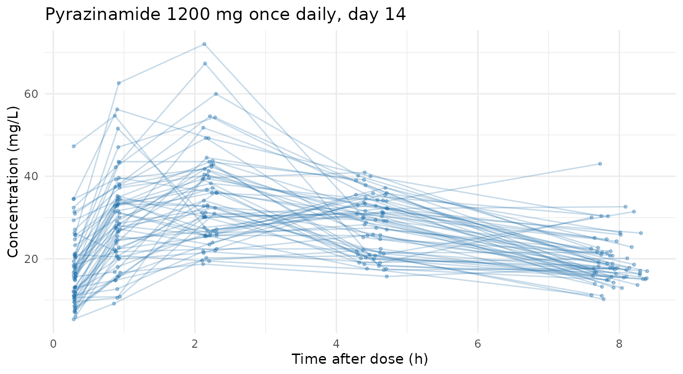
What this does and does not represent
Prior-only generation exists to produce structurally correct data for pipeline and model-code development. It is not a reimplementation of the source model, and three parts of the specification have no representation in it. None of them fails loudly, so they are listed here rather than left to be discovered.
1. Covariate effects, which is why no covariates are generated
The requested WT exponents (0.75 on CL/F, 1 on V/F), the GENDER effect on CL/F (-0.40), and the CD38 effect on CL/F (-0.22) have nowhere to go.
The reason is not a deep one. The generator draws each subject’s
parameters as typical value times lognormal IIV and simulates the whole
profile from those. Covariates, when requested, are drawn separately
afterwards and merged onto the finished table, so by the time a weight
exists the concentration beside it has already been computed. No
argument on pmx_structural_model() links them, and no code
in the package applies a covariate to a parameter.
The generator will happily add the columns if asked, and
pmx_covariates_reference() makes that a single call:
pmx_covariates_reference(c(WT = "WT", GENDER = "SEX"))
#> Covariates
#>   WT: continuous [35, 180]; lognormal, median 84, CV 25% (public, DP)
#>   GENDER: categorical {M 50%, F 50%} (public, DP)
Those are plausible numbers bearing no relationship to the concentrations in the same row, and a reader who did not know that would draw a false conclusion from the first covariate plot they made. A missing column is honest and a meaningless one is not, so they are left out here. Add them only if your pipeline needs columns of the right type to run against, and say so where anyone might read them otherwise.
Note what this is not. It is not a privacy constraint:
prior-only generation reads nothing, so a covariate effect would be a
public assertion exactly like typical and iiv,
costing no budget. (In the differentially private engines the calculus
differs, since every covariate consumes a slice of the budget.) It is
simply unimplemented. If you need covariate-parameter relationships,
simulate them explicitly in rxode2 or nlmixr2,
or use synpmx_avatar() on real data, where real covariate
relationships survive because whole real subjects do.
2. Inter-occasion variability is absent
The requested inter-occasion variability on V (log-SD 0.117) is not represented; the generator draws one parameter vector per subject for the whole study. With sampling on a single day this is a small omission here, but it would matter if the schedule were extended across occasions.
3. Residual error is proportional only
residual_cv = 0.22 carries the proportional part. The
additive component (SD 2.41 mg/L) has no argument and is dropped, so low
concentrations are less noisy than specified. With sampling ending at 8
h and concentrations staying well above the additive scale the practical
effect is modest, but at a trough it would not be.
What the output is good for: exercising code that reads, reshapes, plots and fits a repeated-dose PK dataset with a realistic event structure, nominal and actual times, occasions, and a censoring flag, without a single real patient being involved.
Where to go next
-
vignette("prior-algorithm")— what the generator does with these inputs, and the full catalogue of models and designs it can express. - Calibration — the same public model, with a small privacy budget spent correcting its magnitude against a real study.
- Building the structural model and Describing the trial — how to produce the two public inputs above without reading data.
- The synpmx data generation algorithms — the other generation modes, and which one to use when.